Follow the presentation on your device

https://phd-defense.pau.engineer

Scan the QR code

Personal & Institutional Context

• University Teacher Training Fellowship FPU20/05700 (2021–2025);
  ≈180 hours of teaching microwave and electronics labs & problem solving
• Research stay: University of British Columbia in Canada (AI-enabled sensing)
• Industry Projects:
  • Smart Cellar CPP Project (Garcia Carrion)
  • Corrosion detection in urban lighting poles (RUBATEC)
• National Research Projects:
  • PID2019-103904RB-I00 (Design and synthesis of RF/microwave devices...)
  • PID2022-139181OB-I00 ($\mu$WAVE-SENS)
• External Projects:
  • AI4ALL 2023 Winner team (Real world applications of AI)
  • AI Accelerator 2023 Mobile World Congress (Continuation of AI4ALL)
• Outcomes: thesis contributions (11 compendium articles + 7 works) + tech transfer (agrifood, structural health monitoring, future hospital pilots)

Outline

• I. Thesis Objectives
• II. Fundamentals
• III. Sensitivity Enhancement
• IV. AI-Driven Sensing
• V. Applications & Discussion
• VI. Future Work & Conclusions

The Problem: Sensitivity vs Selectivity

Analogy: Smoke Detector

Sensitive to smoke (toast or fire?)

Discern type of smoke

The Goal: Sensitive & Selective Sensing

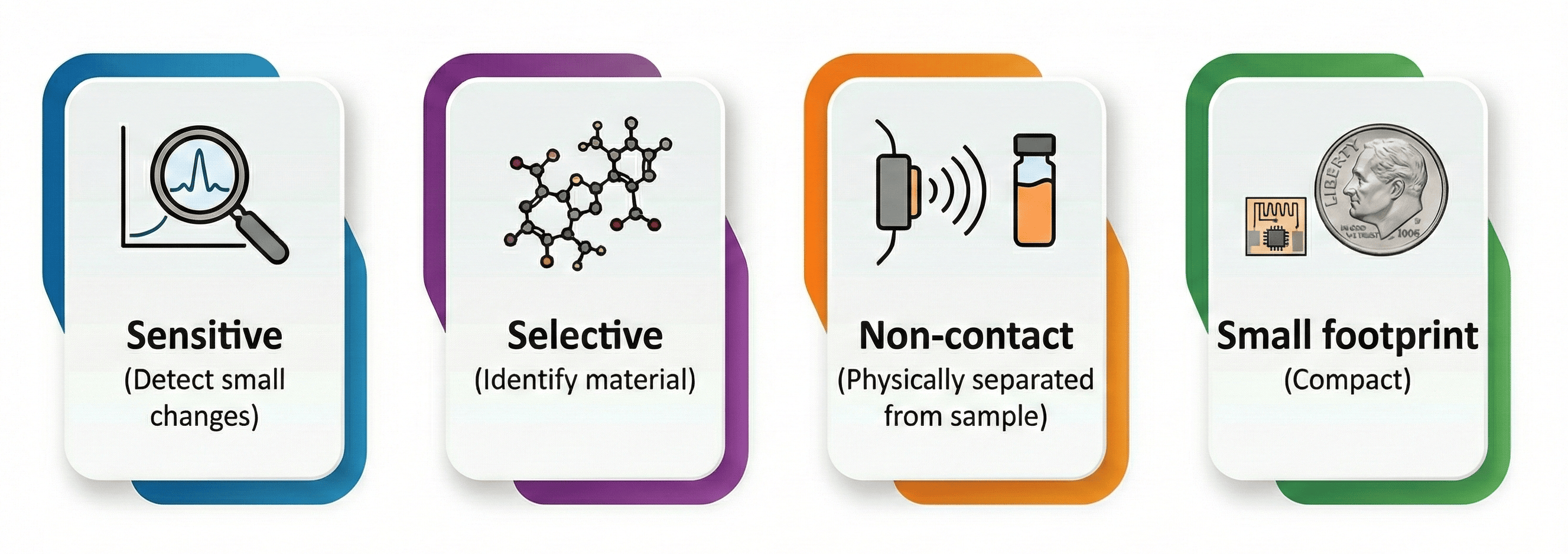
Thesis Objectives

1. Sensitivity & Size Optimization
   Maximize sensitivity per unit area.
2. Liquid Measurement & Automation
   Reliable characterization of fluids.
3. AI-Enabled Sensing Modalities
   Selectivity and remote sensing via ML.

Planar Technology

Guiding Waves

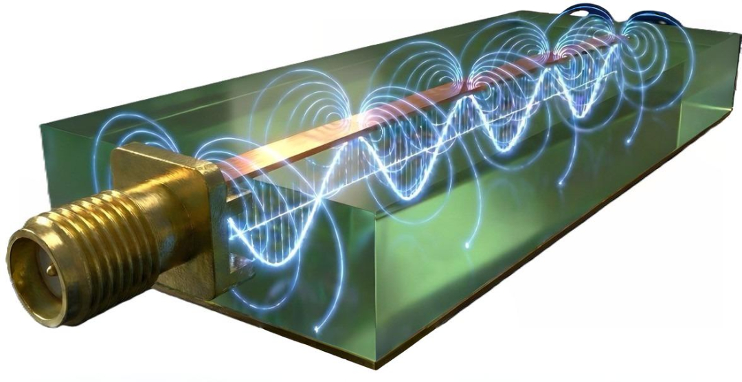
• Microstrip & CPW lines
• Confines field to a specific region

Benefits

• Controllability
• Low Cost
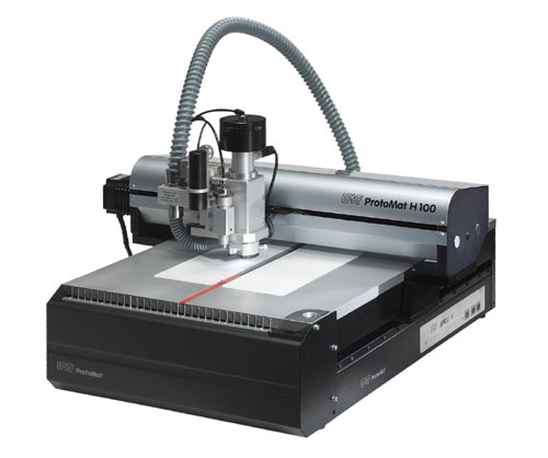
• Easy Fabrication (CNC)

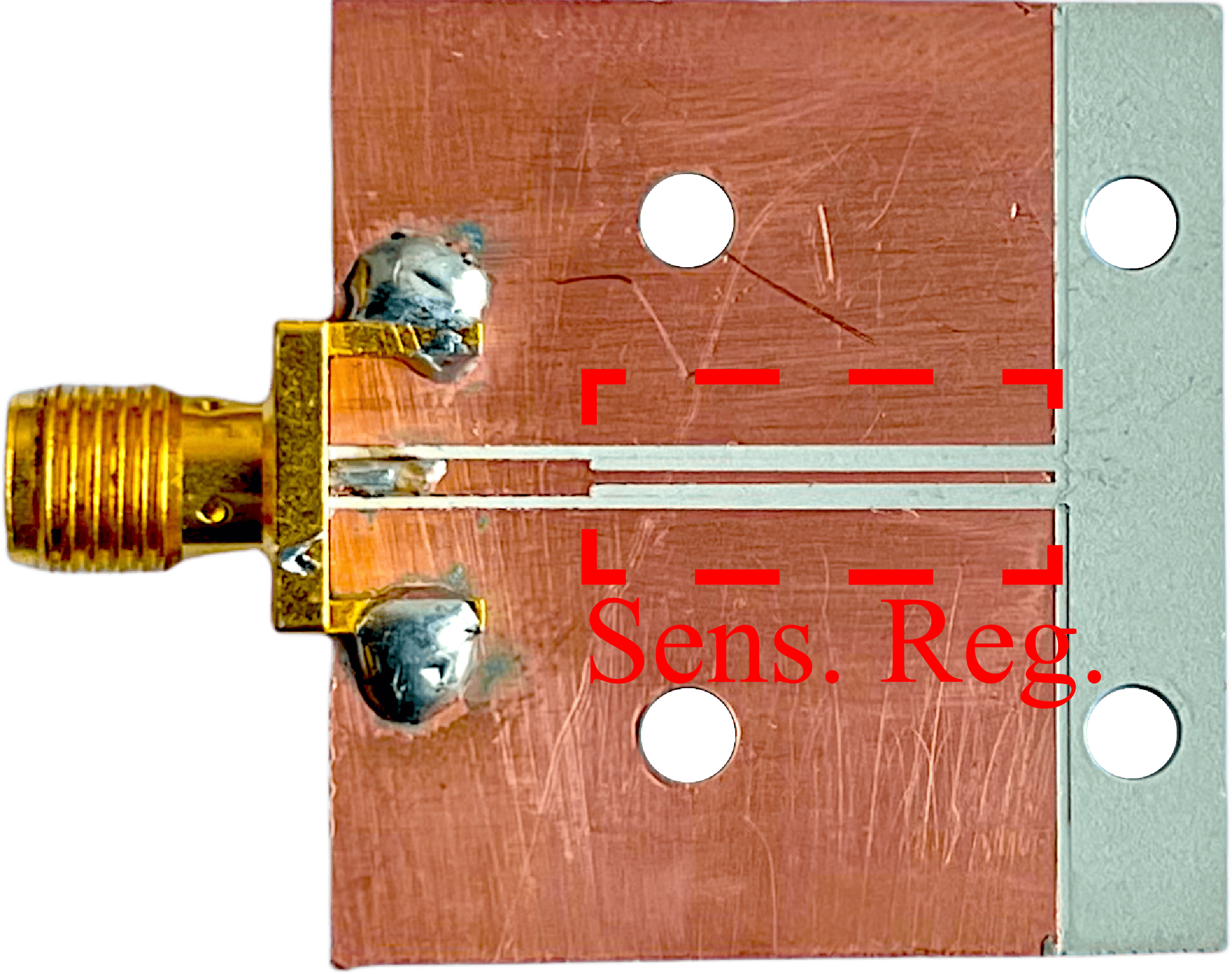
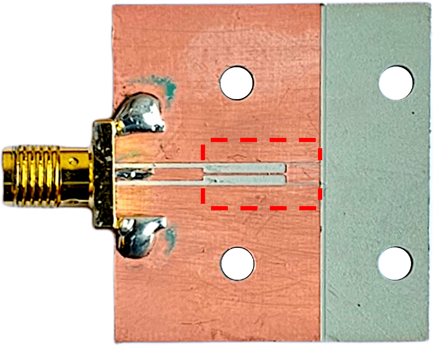
Resonators

• Sensing Region: Where field interacts with MUT (Material Under Test).
• Resonance: High sensitivity to dielectric changes.
• Topology: Can be shaped to optimize interaction.

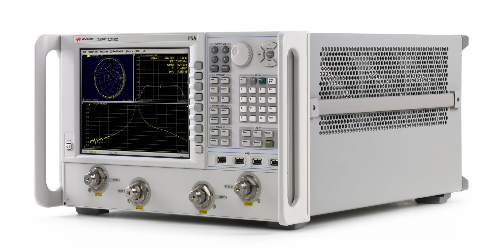
Measurement: VNA

• Vector Network Analyzer (VNA): The "instrumental" part of the measurement.
• Function: Generates signal and analyzes reflection and transmission.
• Parameter: Reflection ($\rho$) and Transmission ($\tau$) Coefficients.

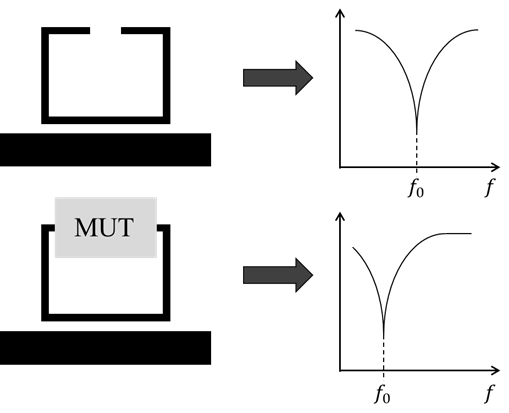
Frequency Variation Sensors

• Principle: Resonance frequency shift caused by MUT.
• Pros: Simple structure but complex readout.
• Cons: Spectrum analysis required for measurement.

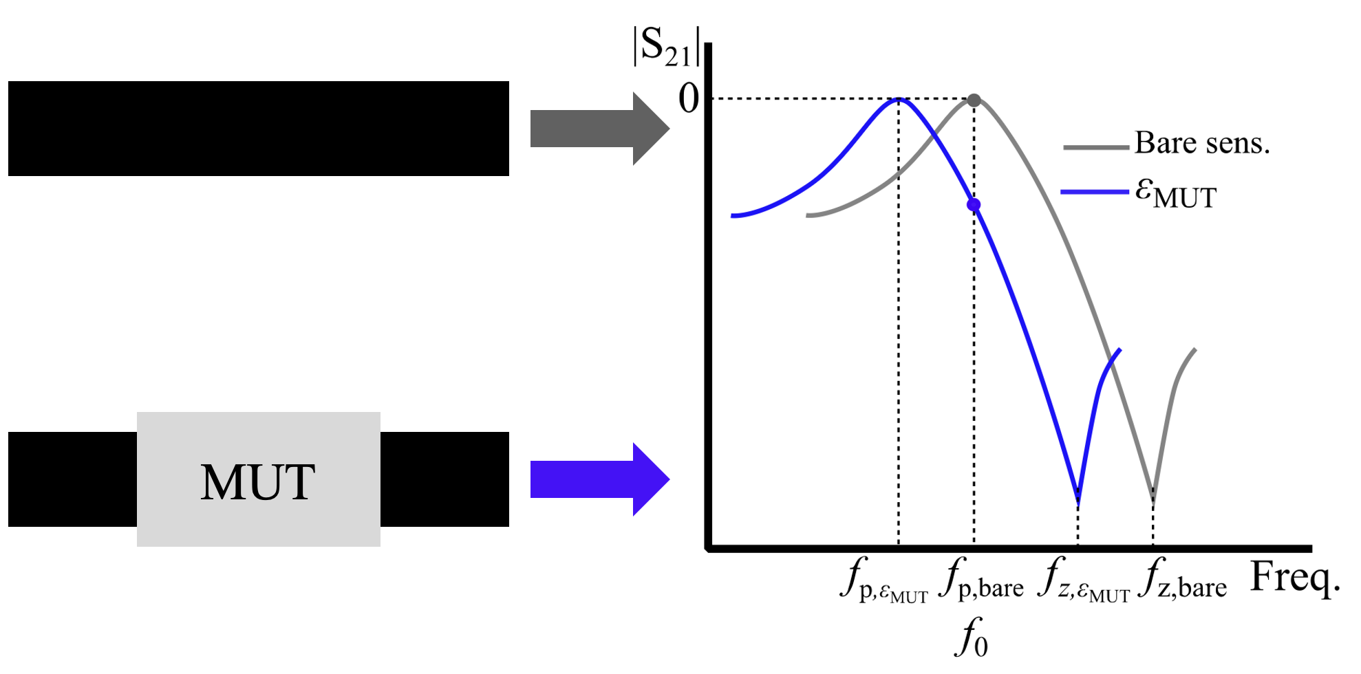
Magnitude Variation Sensors

• Principle: Variation in Q-factor or peak/notch attenuation.
• Pros:
  • Simple scalar readout.
  • Single frequency operation.
• Cons: Susceptibility to noise.

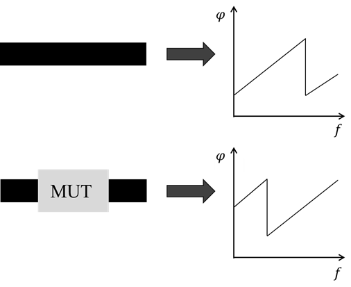
Phase Variation Sensors

• Principle: Phase shift at a single frequency.
• Pros:
  • Single frequency operation.
  • Robust against EMI.
• Cons: Trade-off between size and sensitivity (requires long lines).

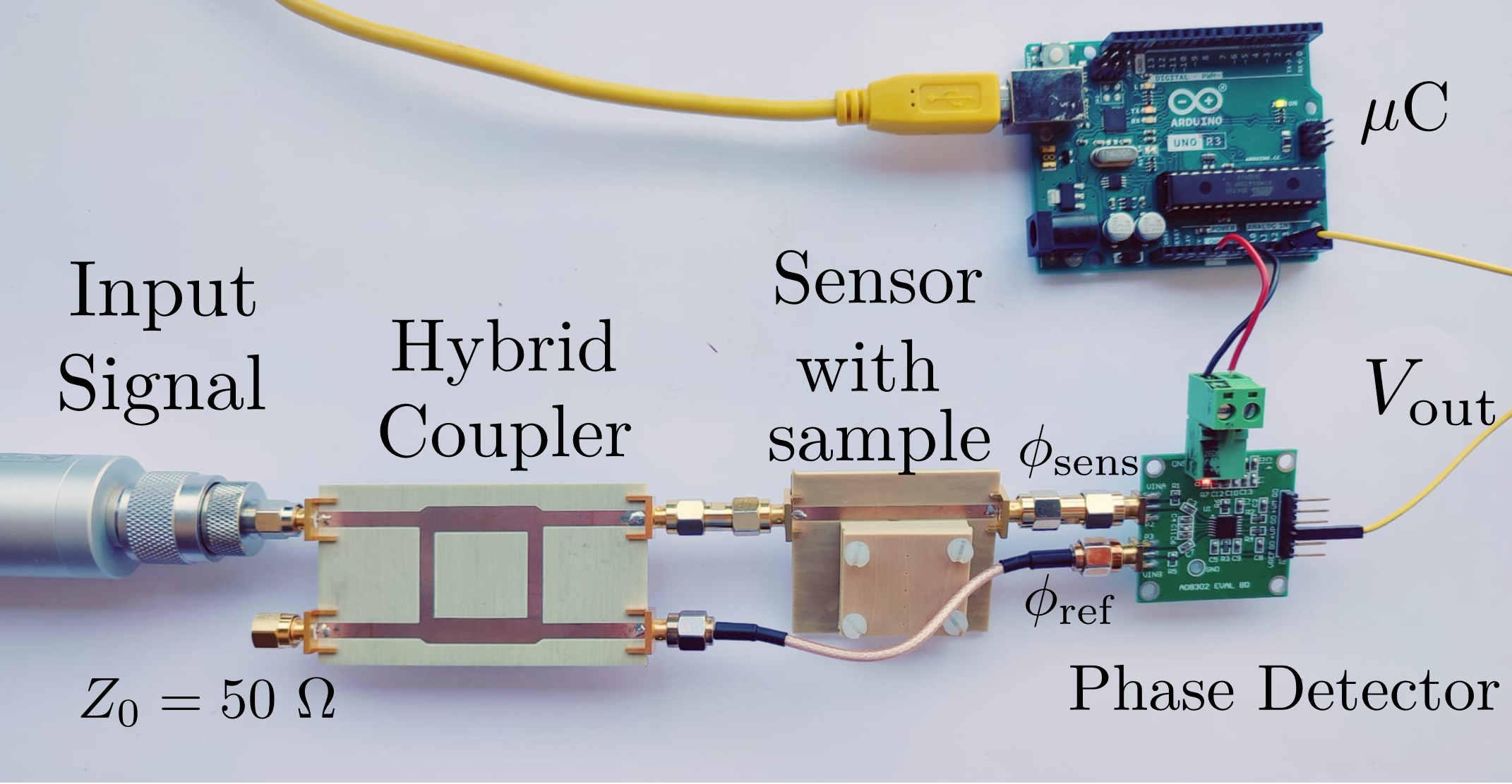
Readout Strategy

• Single Frequency Operation:
  • Focus on one frequency where sensitivity is highest.
  • Reduces readout complexity and cost.
• Accessibility:
  • From Lab Equipment to Portable Devices (LiteVNA ~100€).
  • Low cost phase detector (AD8302 ~5€).

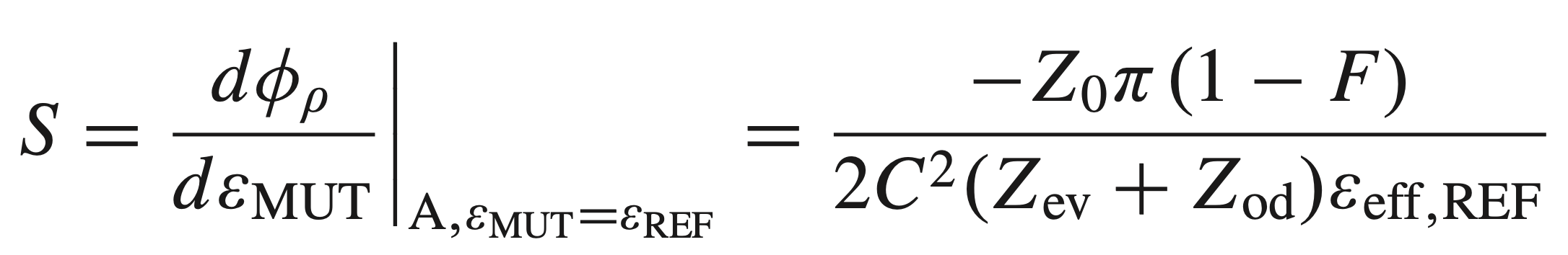
Defining Sensitivity

Sensitivity ($S$) is defined as the change in the phase of the reflection coefficient ($\phi_\rho$) per unit change in permittivity ($\varepsilon_\mathrm{MUT}$).

$ S = \frac{d\phi_\rho}{d\varepsilon_\mathrm{MUT}} $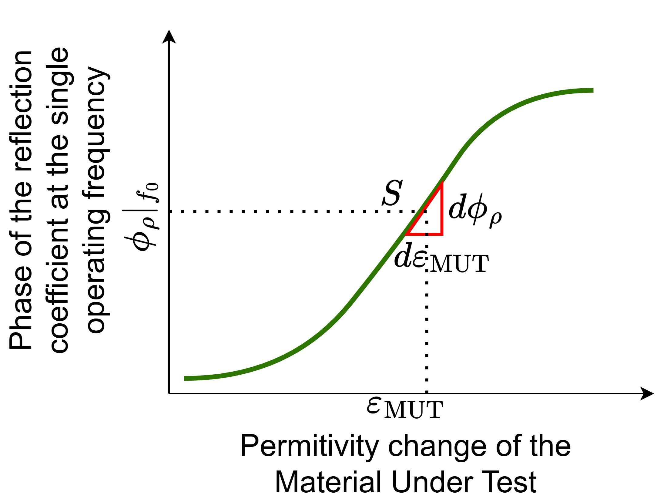

Sensitivity Decomposition

We can decompose sensitivity into two independent factors:

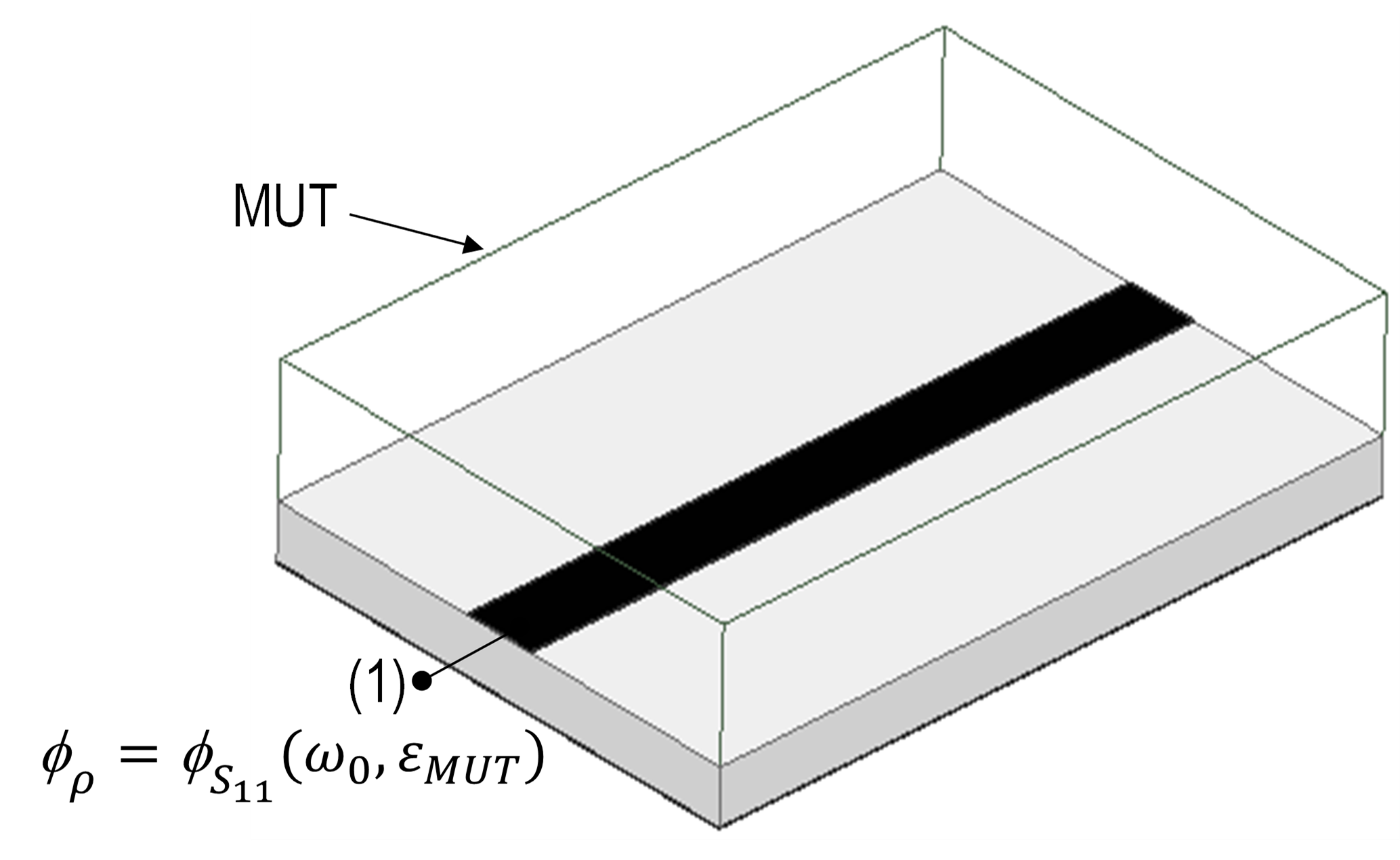
Field Interaction ($\frac{d\upsilon}{d\varepsilon_{MUT}}$)

• Physics: How the electric field penetrates the material.
• Optimization:
  • Maximize field concentration.
  • Use thin substrates or CPW structures.

Electrical Transformation ($\frac{d\phi}{d\upsilon}$)

• Circuit: How the sensor circuital elements converts parameter change to phase shift.
• Optimization:
  • Phase Slope Enhancement Techniques.
  • This is the term where we can gain orders of magnitude!

Four Ways to Increase Sensitivity

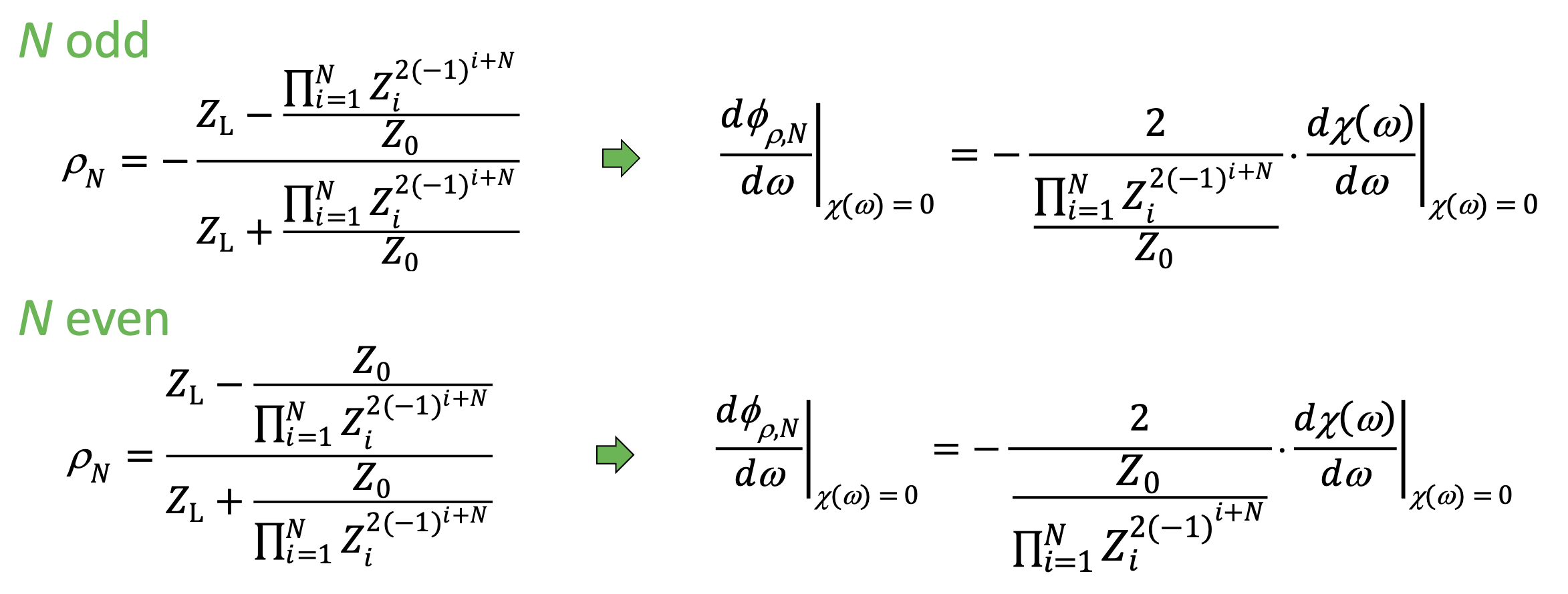
1. High/Low Impedance Inverters

Concept: Cascading 90° transmission lines (inverters) with high/low impedance to multiply the phase slope.

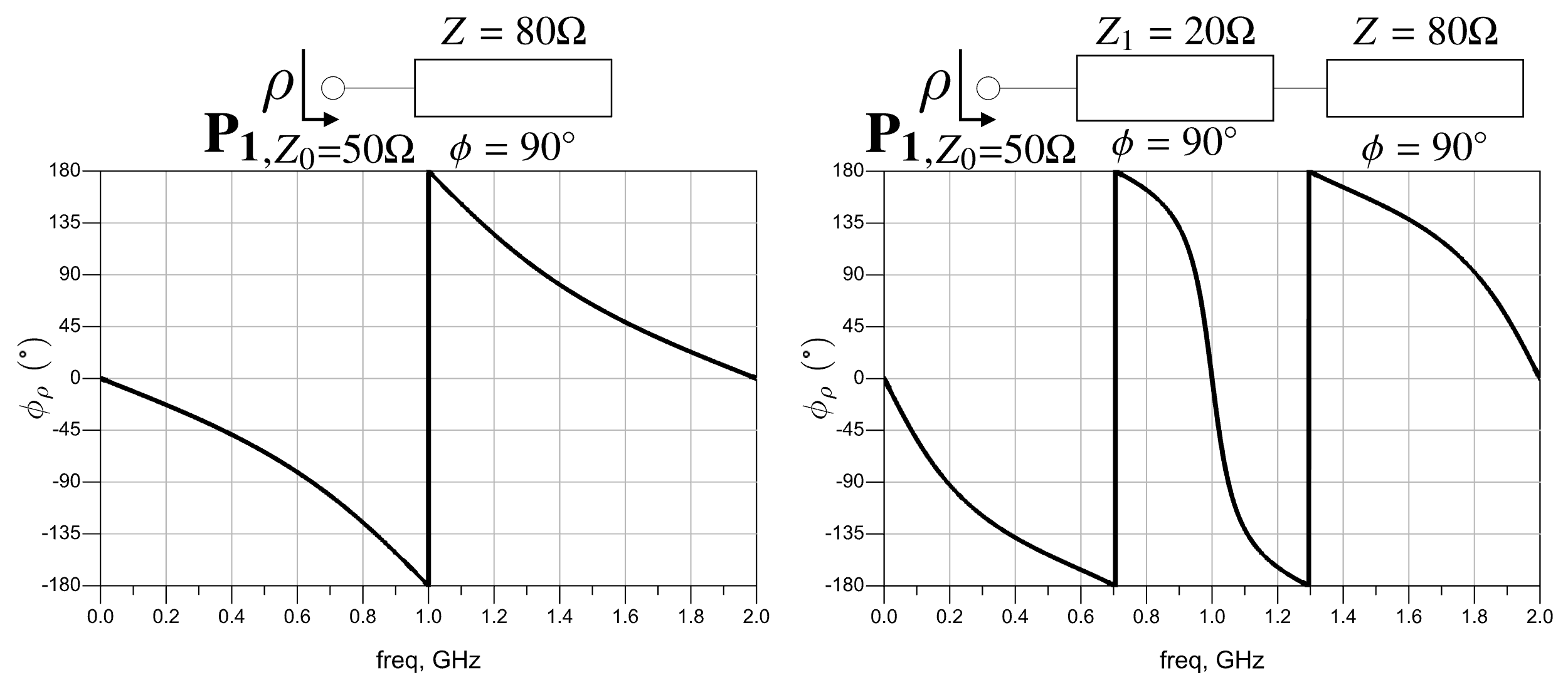
Inverters: Implementation

• Structure: Stepped Impedance Resonator (SIR) + Inverters.
• Goal: Reduce size while maintaining the "multiplied" slope.
• Result: High sensitivity in a compact footprint.

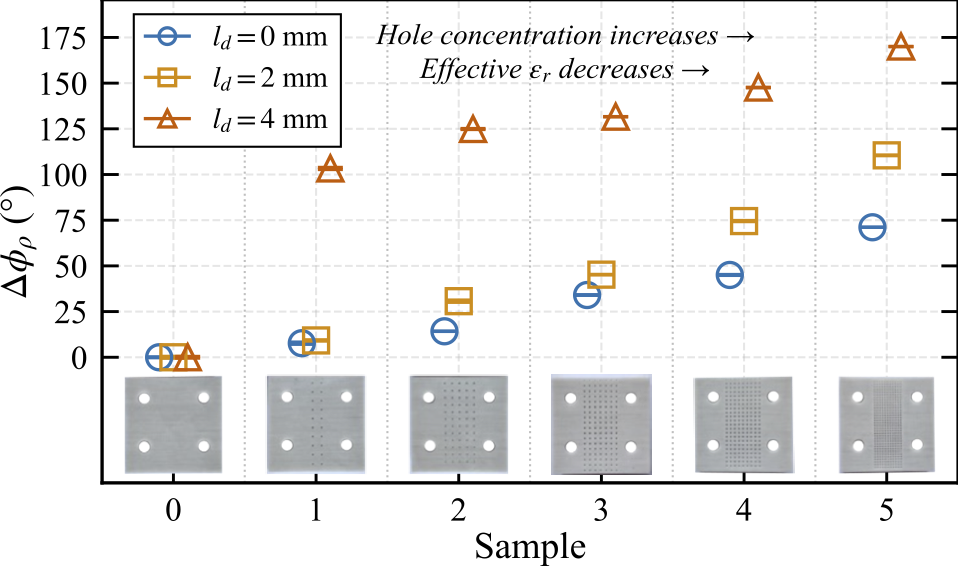
Inverters: Results

• Validated with perforated dielectric samples.
• Outcome: Sensitivity scales with the number of inverters.
• Limitation: Size grows with each inverter stage.

2. Coupled Lines & SIRs

Concept: Two resonators coupled together create two split frequencies.

Reducing coupling $\rightarrow$ Resonances get closer $\rightarrow$ Steeper Phase Slope.

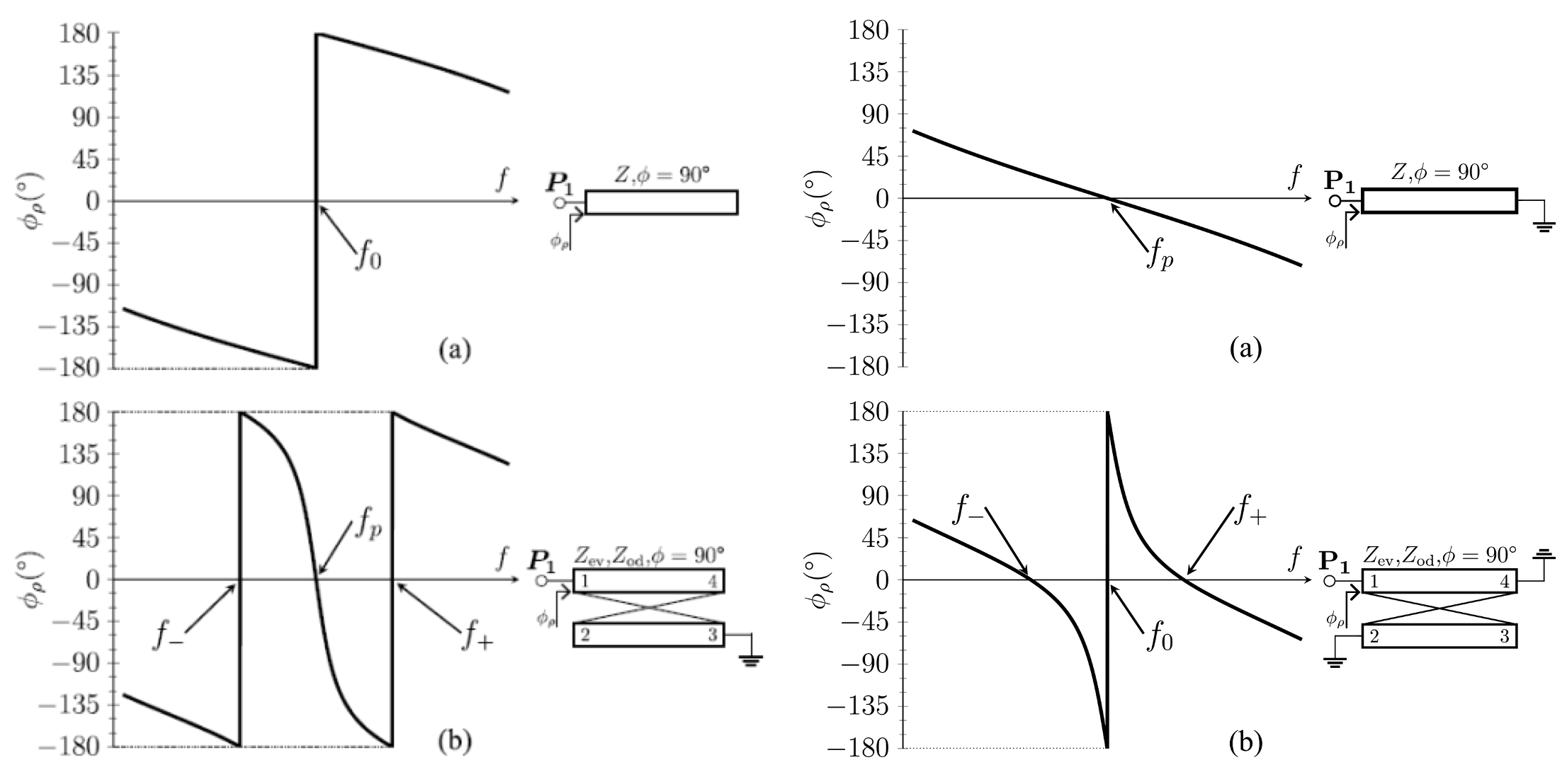
The Coupling Effect

• Strong Coupling: Peaks far apart, shallow slope.
• Weak Coupling: Peaks close, steep slope.
• Limit: If coupling is too weak, recover the single resonator behavior.

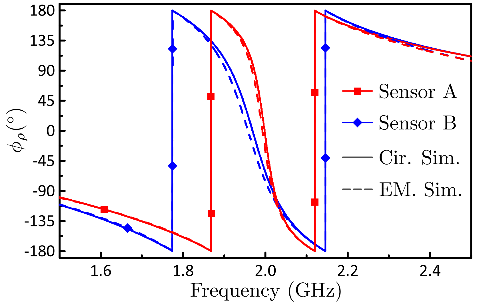
Coupled SIRs Results

• Unified Framework: Analyzed all 4 coupling topologies.
• Achievement: Highest senstivity at the time.
• Publications: 5 compendium papers from this technique.

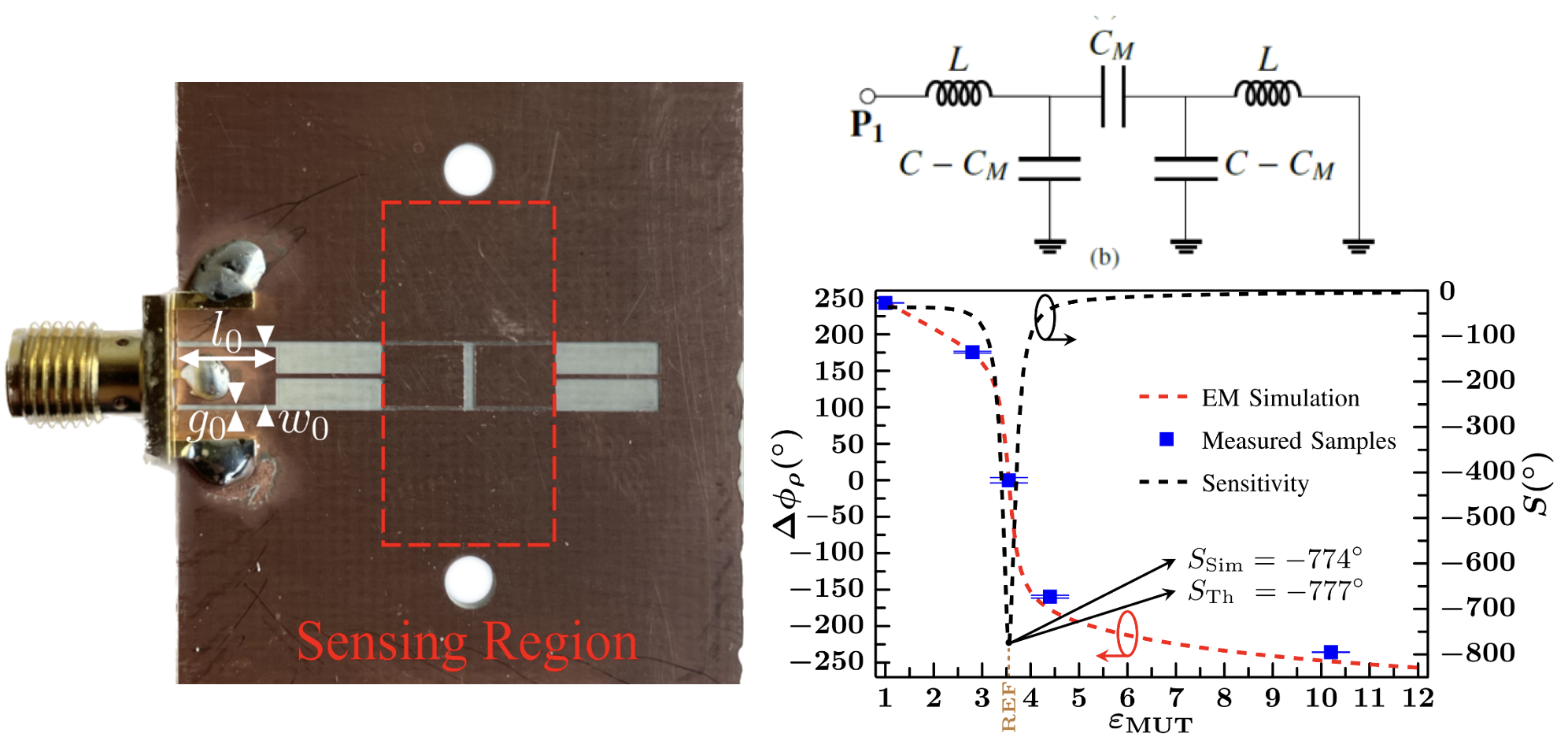
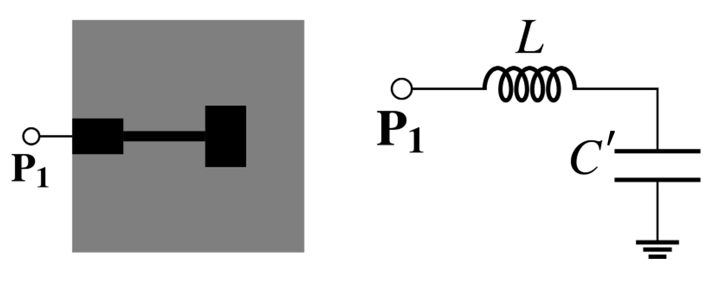
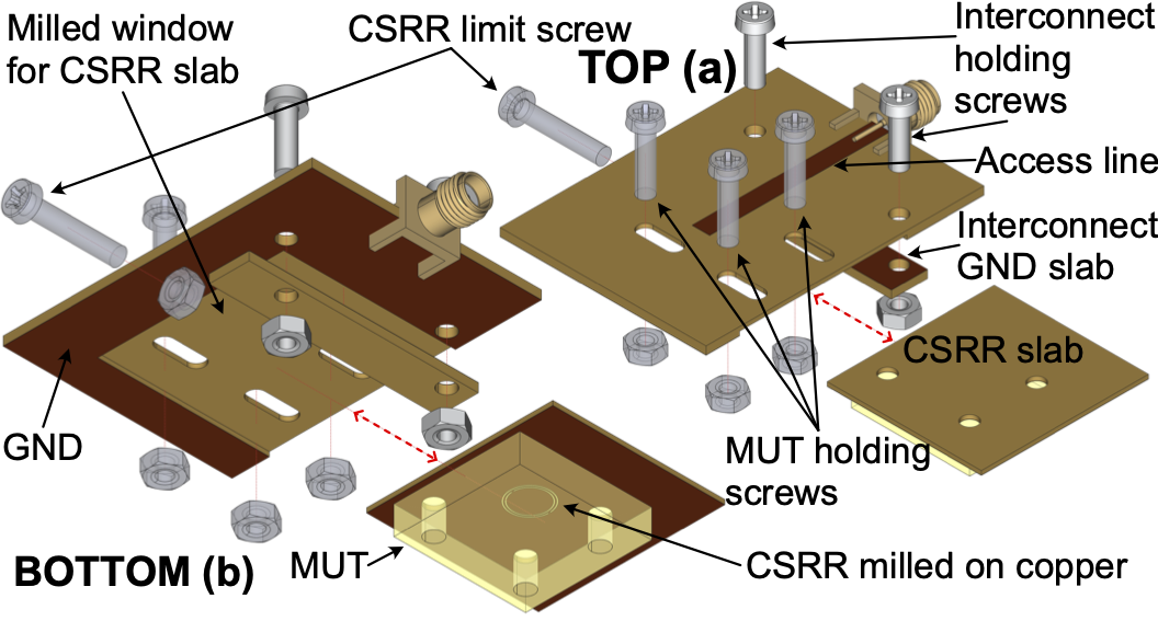
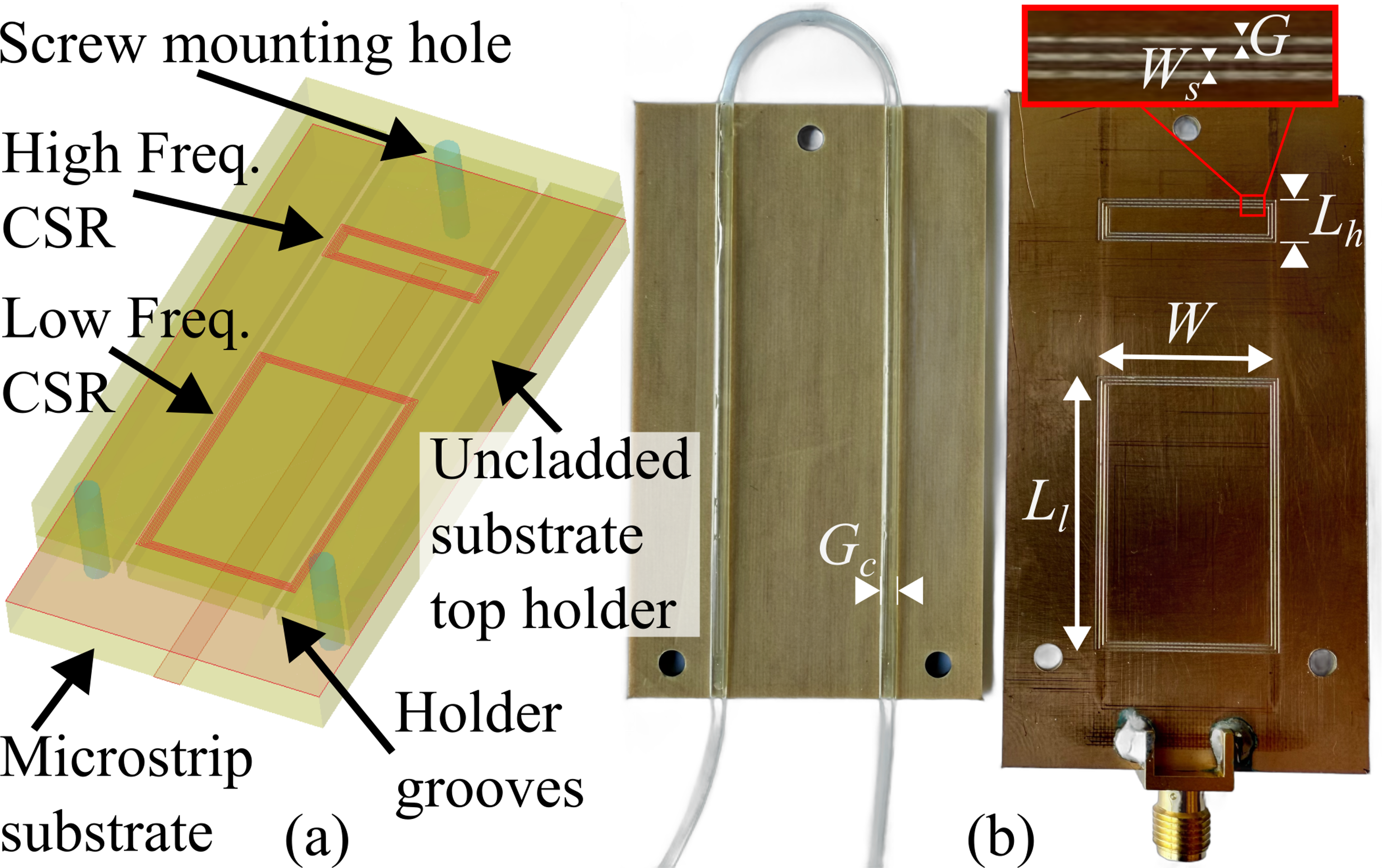
Defect Ground Resonators

Concept: DB-DGS (Dumbbell Defected Ground Structure).

• Separates fluid (ground plane) from circuit (top plane).
• Allows easy integration of fluidic channels.

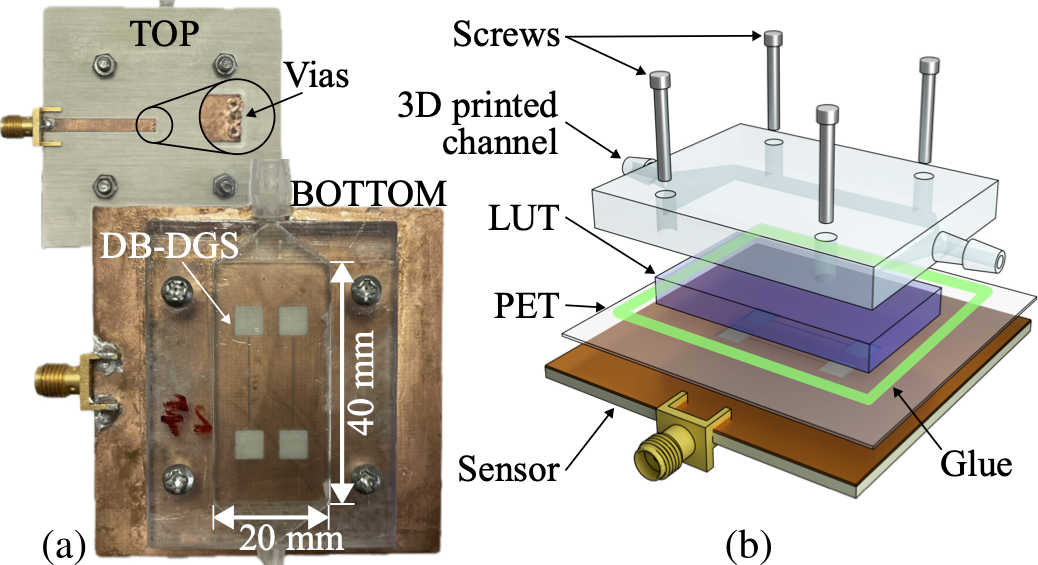
Publication: [pub:DB-DGS]

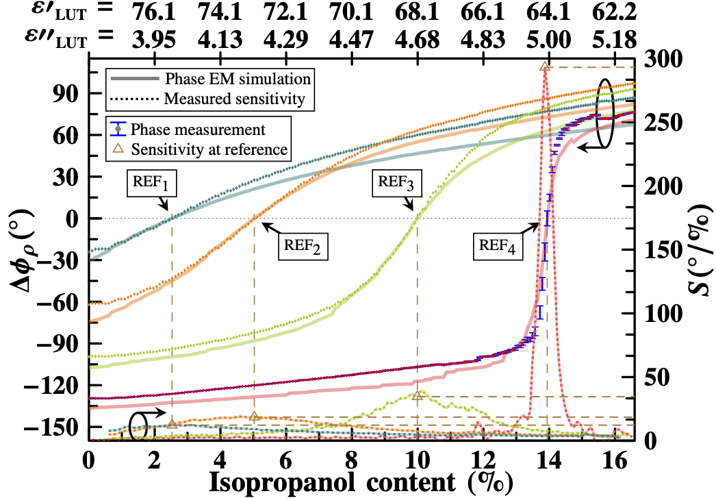
Microfluidics Integration

Challenge: Measuring liquids requires precise handling.

• Liquids allow fine control of permittivity.
• Separate electronics from liquid.
• Need repeatability to validate sensors.

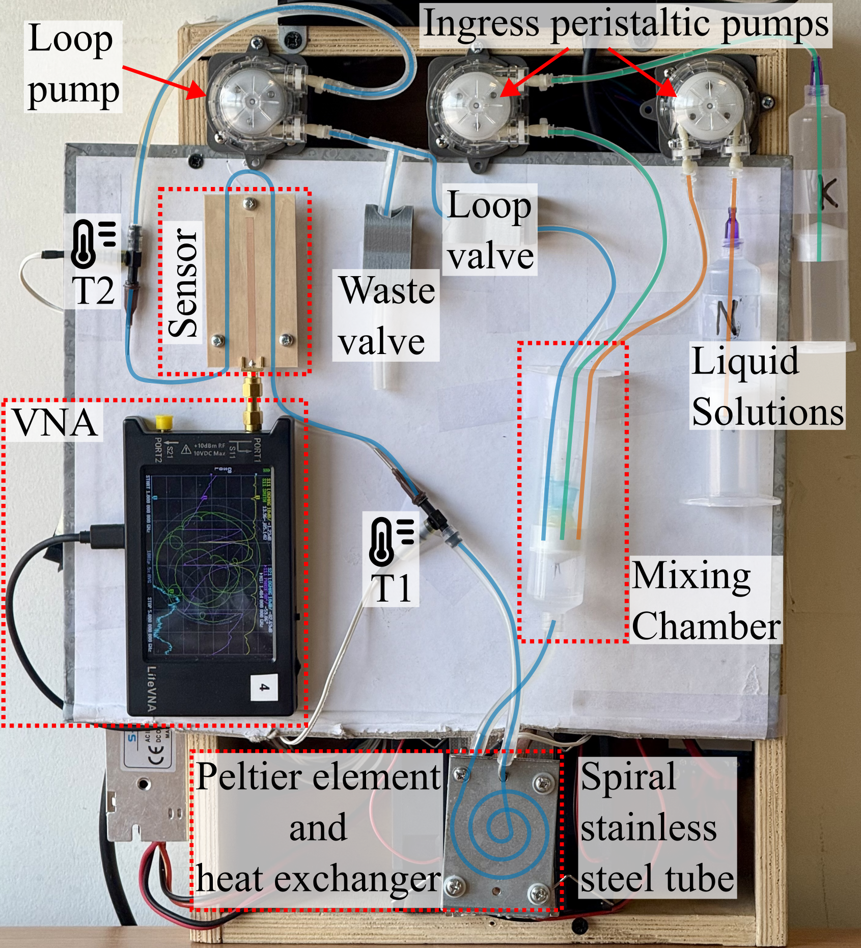
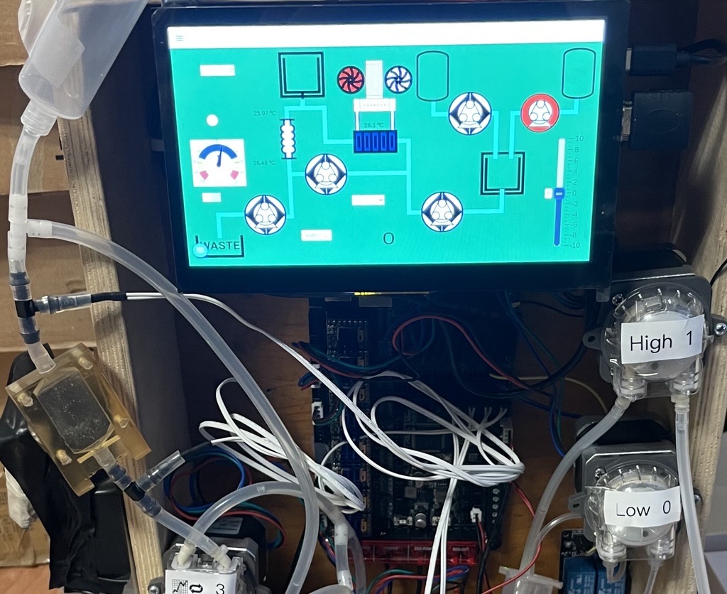
Automated System

• System: Pumps + Temperature Control + VNA.
• Benefit: Automated validation of thousands of samples.
• Key for AI: Enabled generation of large datasets.

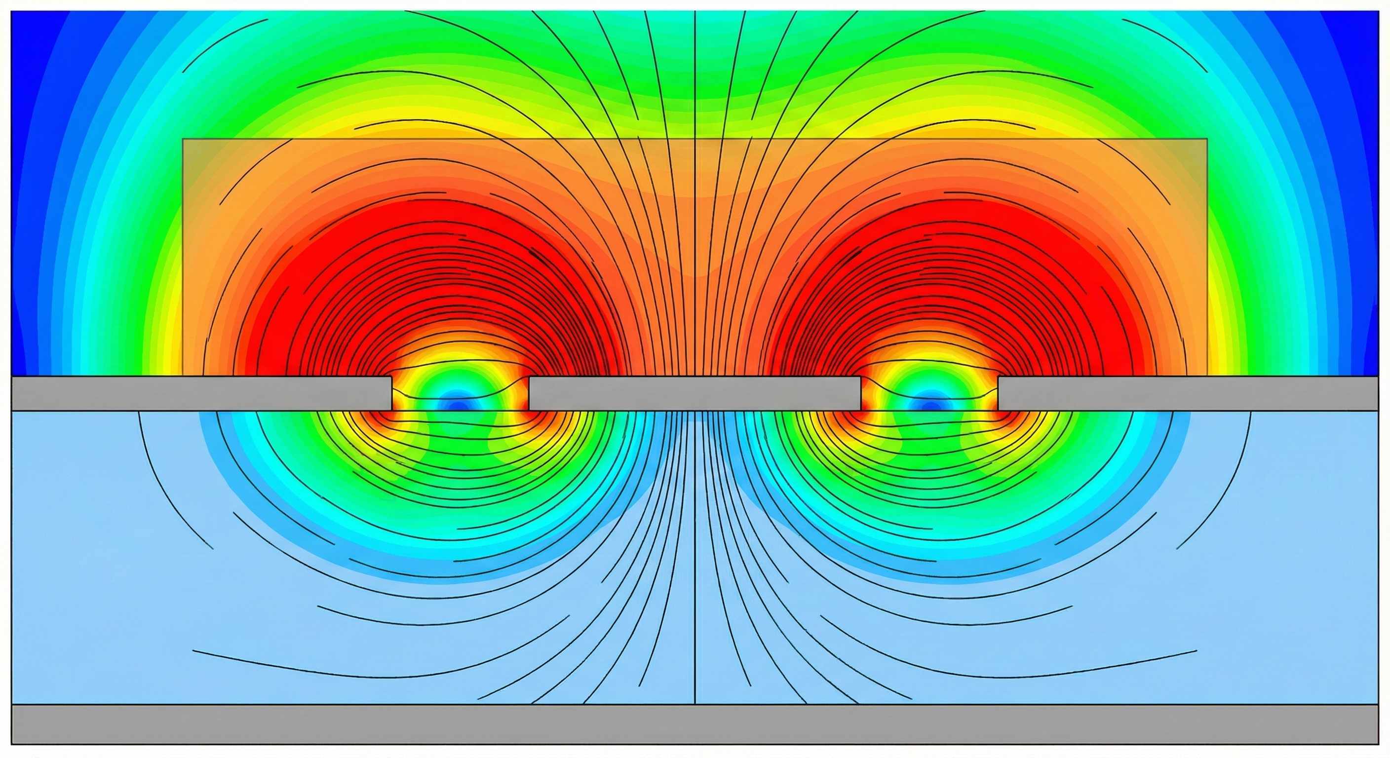
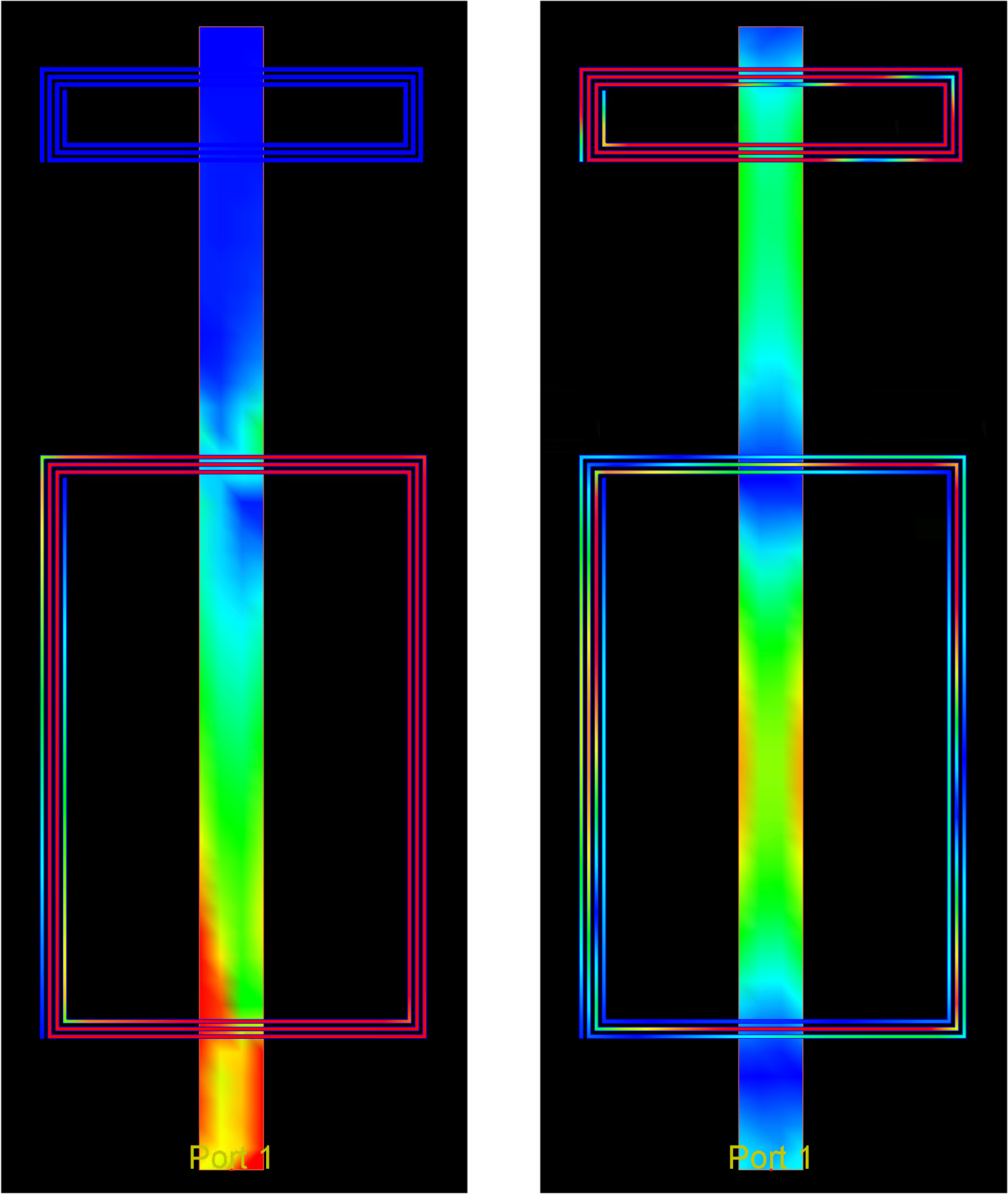
3. Resonance-Antiresonance

Concept: Interaction between a resonance and an antiresonance.

Mechanism: Ground-plane CSRR coupled to a microstrip line, resonance shifts with coupling while antiresonance stays fixed.

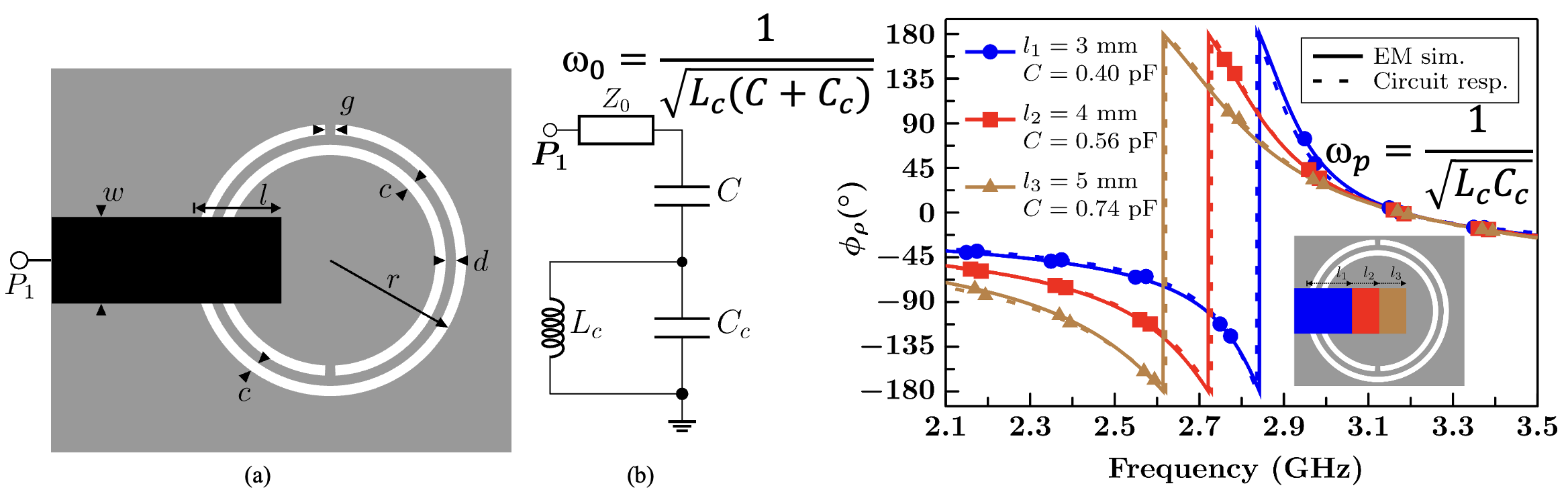
Mechanical Tuning

• Innovation: Sensitivity can be tuned by moving the feed line.
• Benefit: Adapt sensitivity to the application without redesigning.

Results

• Sensitivity: > 6350° per unit permittivity.
• Record: Highest sensitivity achieved in the thesis.
• Application: Structural health monitoring (corrosion) or liquid analysis.

4. Loss Engineering

Paradigm Shift: Instead of minimizing loss, it is a design parameter.

• Concept: Losses can steepen the phase slope near resonance.
• Result: Enhanced sensitivity without changing the geometry.

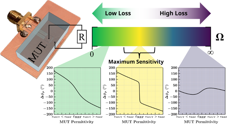
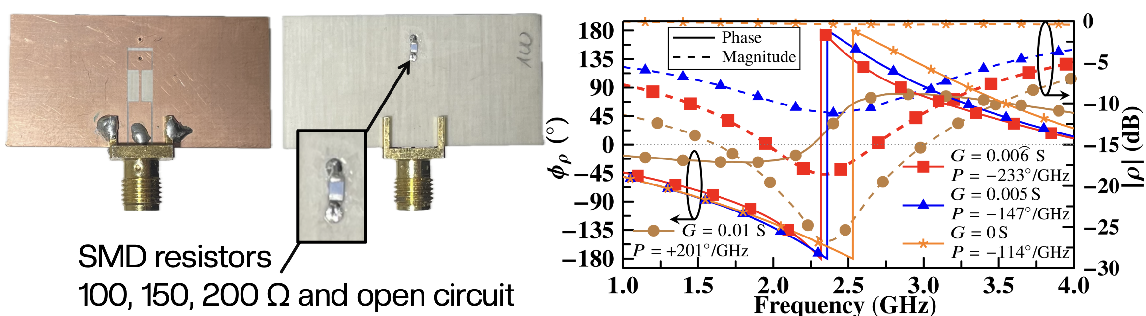
Passive Implementation

Method: Adding resistive loading to coupled lines.

• Mechanism: Resistors control the coupling quality factor.
• Outcome: Steeper phase response in the sensing region.

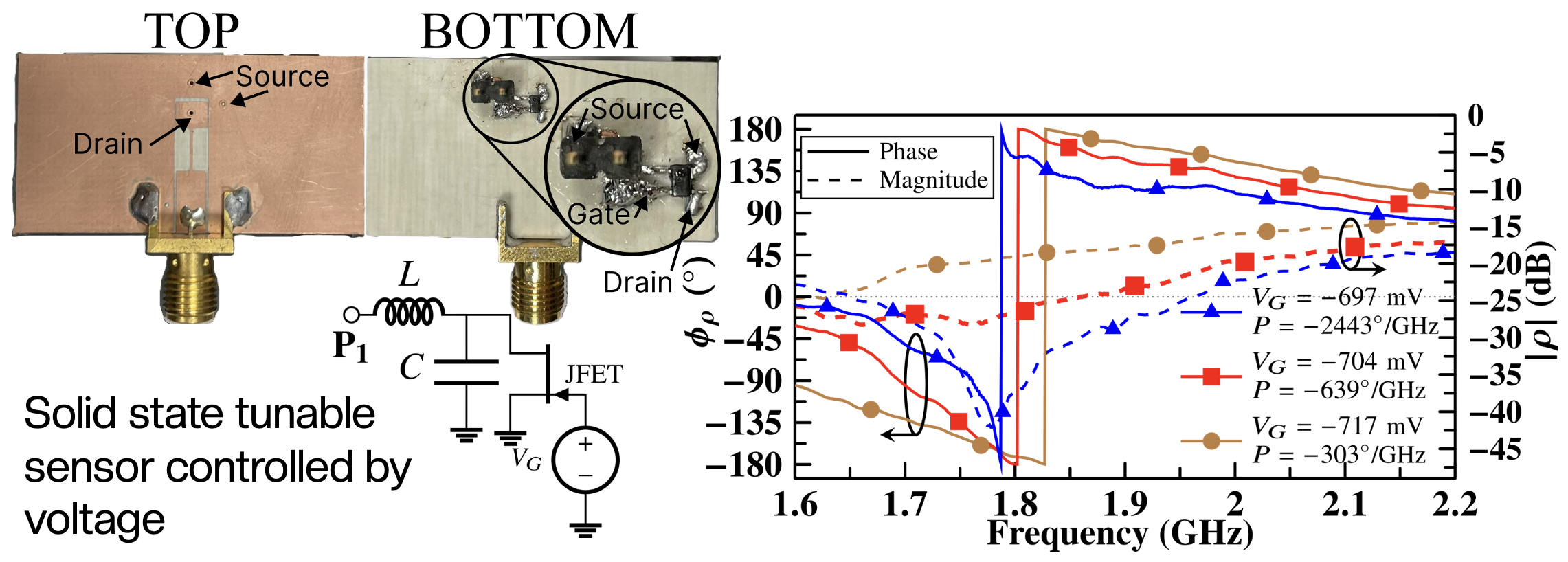
Active Tunable Sensitivity

Method: Using a JFET as a voltage-controlled resistor.

• Innovation: Real-time control of sensitivity.
• Application: Adapt the sensor to different materials dynamically.

The Selectivity Challenge

The Solution: Spectrometry + AI

• Spectrometry: Materials behave differently at different frequencies.
• Broadband Measurement: Capture the "fingerprint" of the material.
• Why AI? Analytical models are too complex for multi-variable inverse problems.
• Traditional design process: Physical Model $\rightarrow$ Analytical Inversion $\rightarrow$ Parameter
• New design process: Data $\rightarrow$ Machine Learning Model $\rightarrow$ Prediction

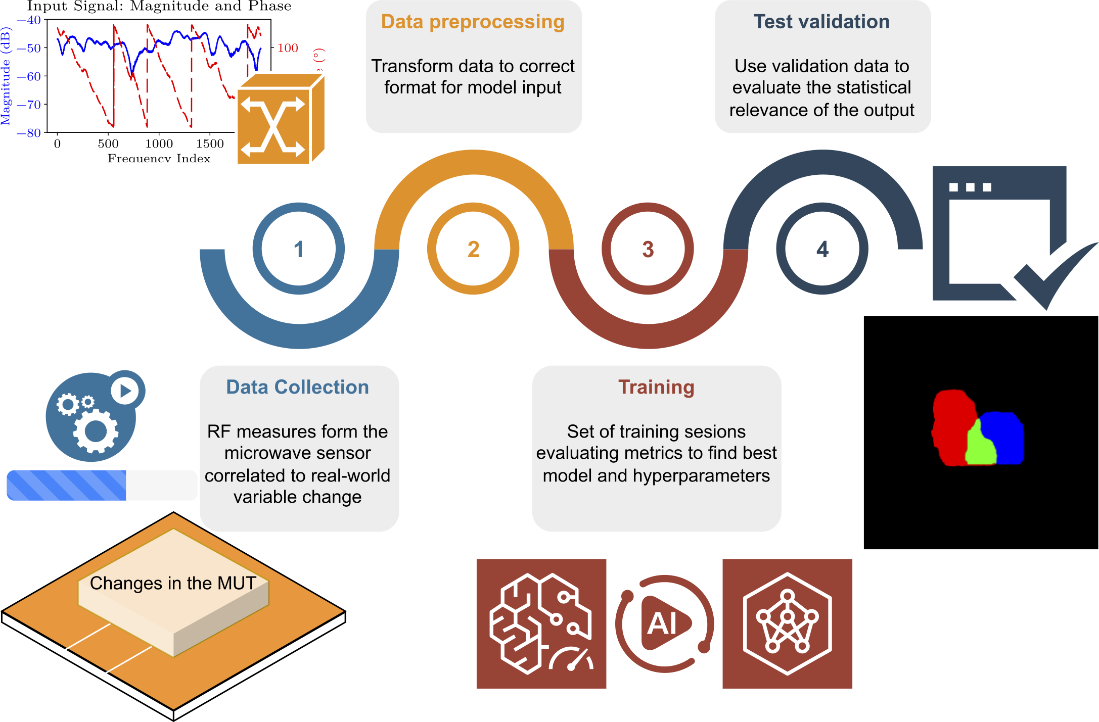
The Pipeline

1. Design Sensor: For contrast, not just sensitivity.
2. Generate Data: Automated measurements / Simulation.
3. Train Model: Learn the mapping (Spectrum $\rightarrow$ Variable).
4. Inference: Real-time prediction.

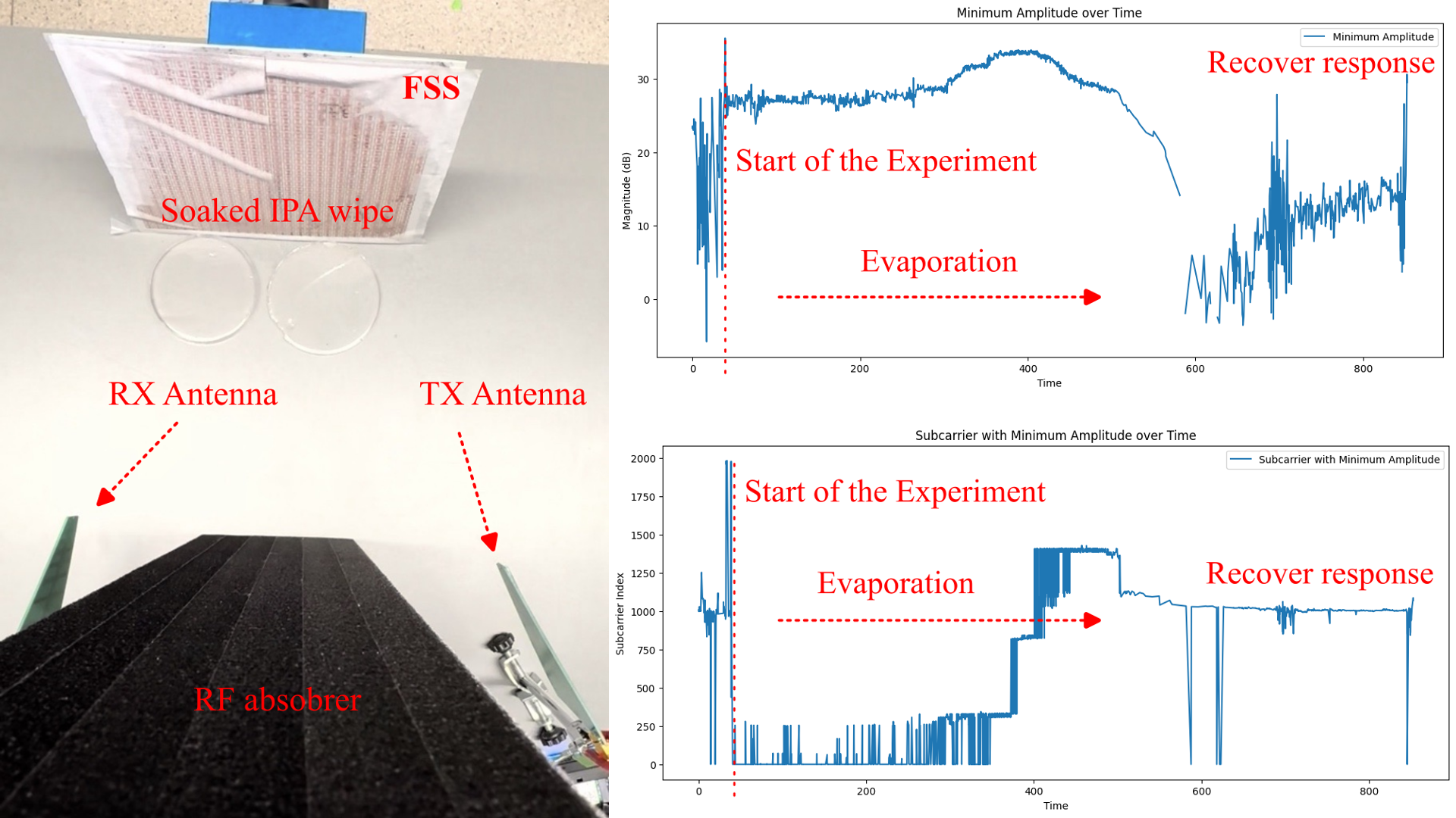
Case 1: Remote Sensing with FSS

Scenario: Detecting liquid spills remotely.

Sensor: Frequency Selective Surface (FSS) tag.

Challenge: Signal depends on liquid type AND position.

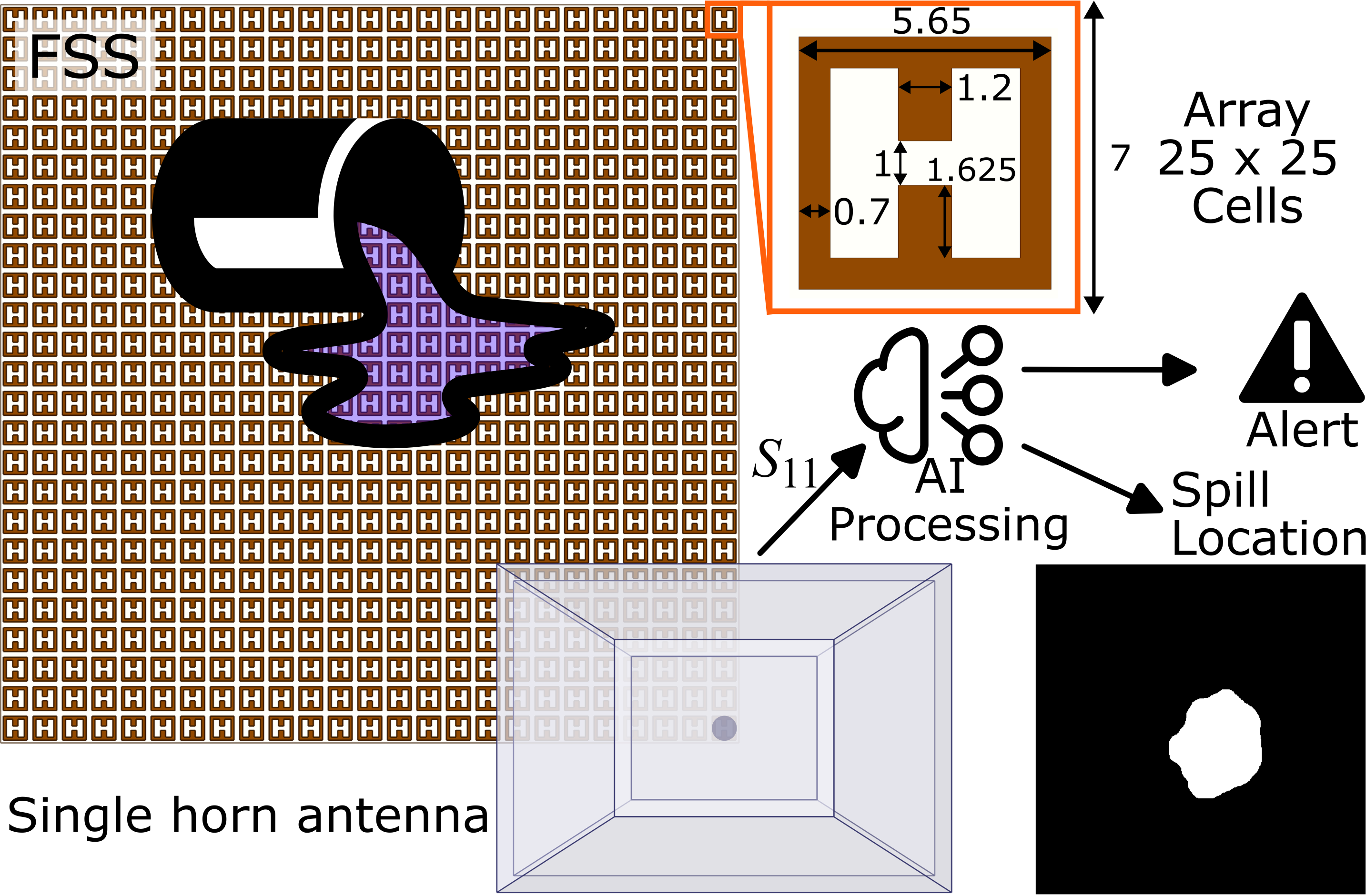
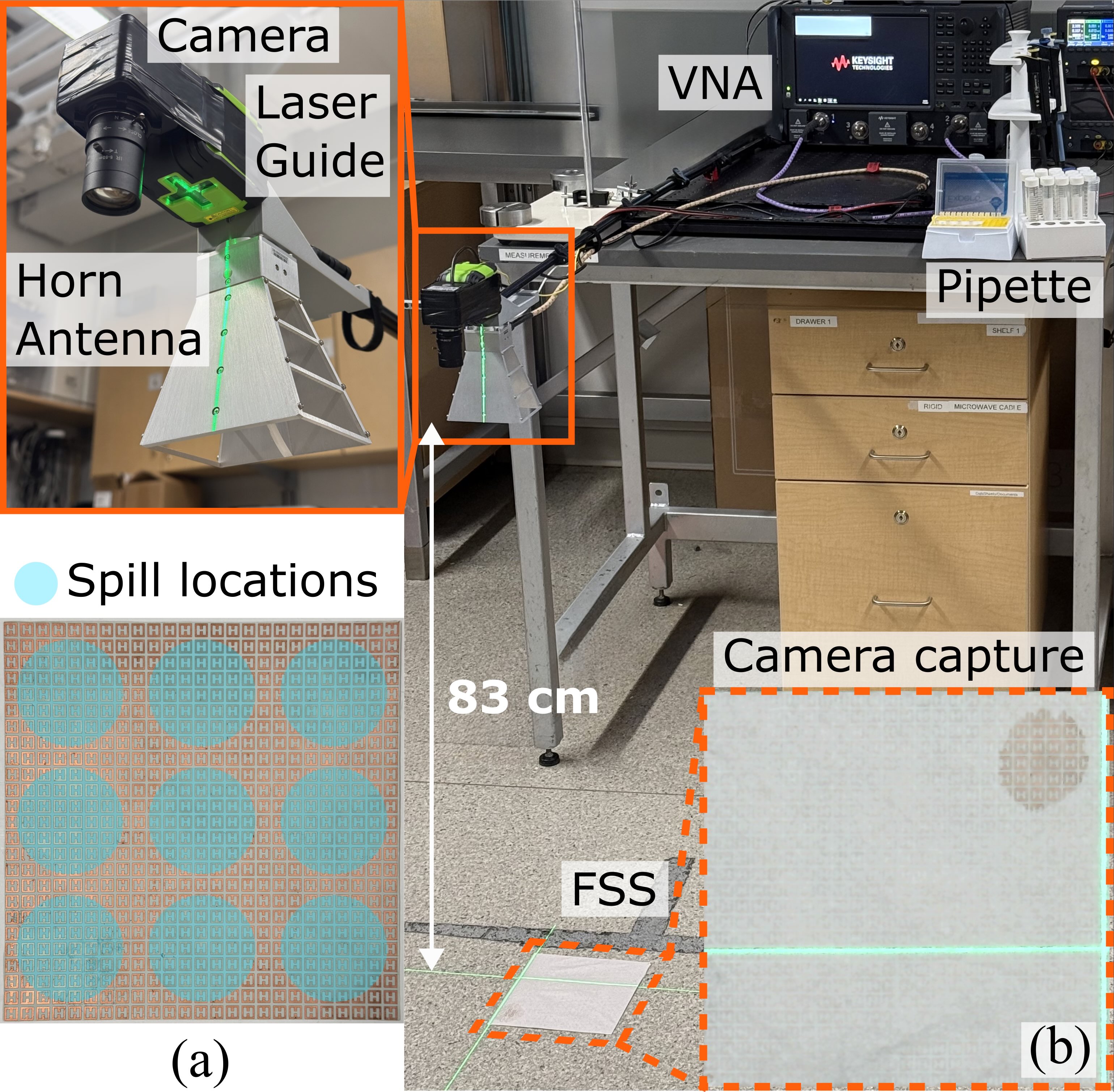
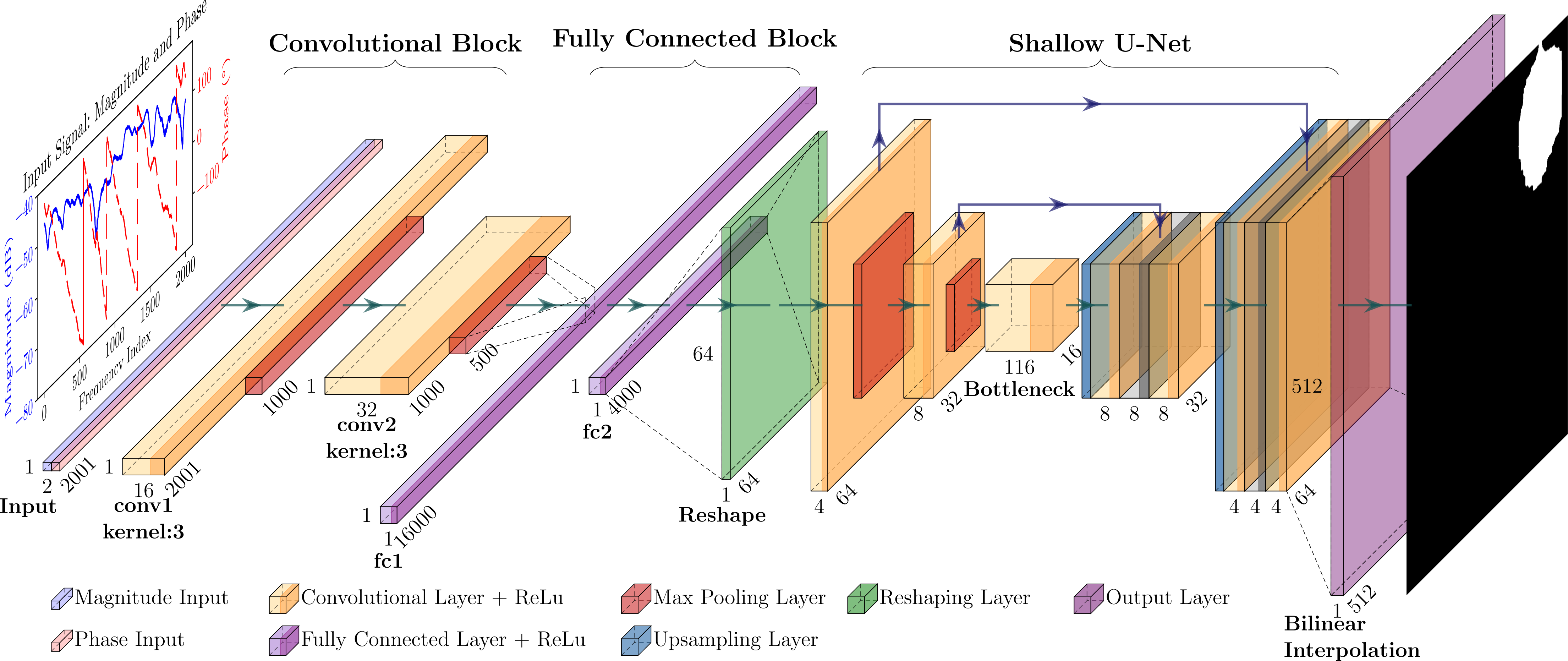
FSS Solution: CNN + U-Net

• Input: Single radar echo (1D spectrum).
• CNN Model: Signal feature extraction.
• MLP Model: Latent space mapping.
• U-Net Model: Spatial Mask reconstruction.

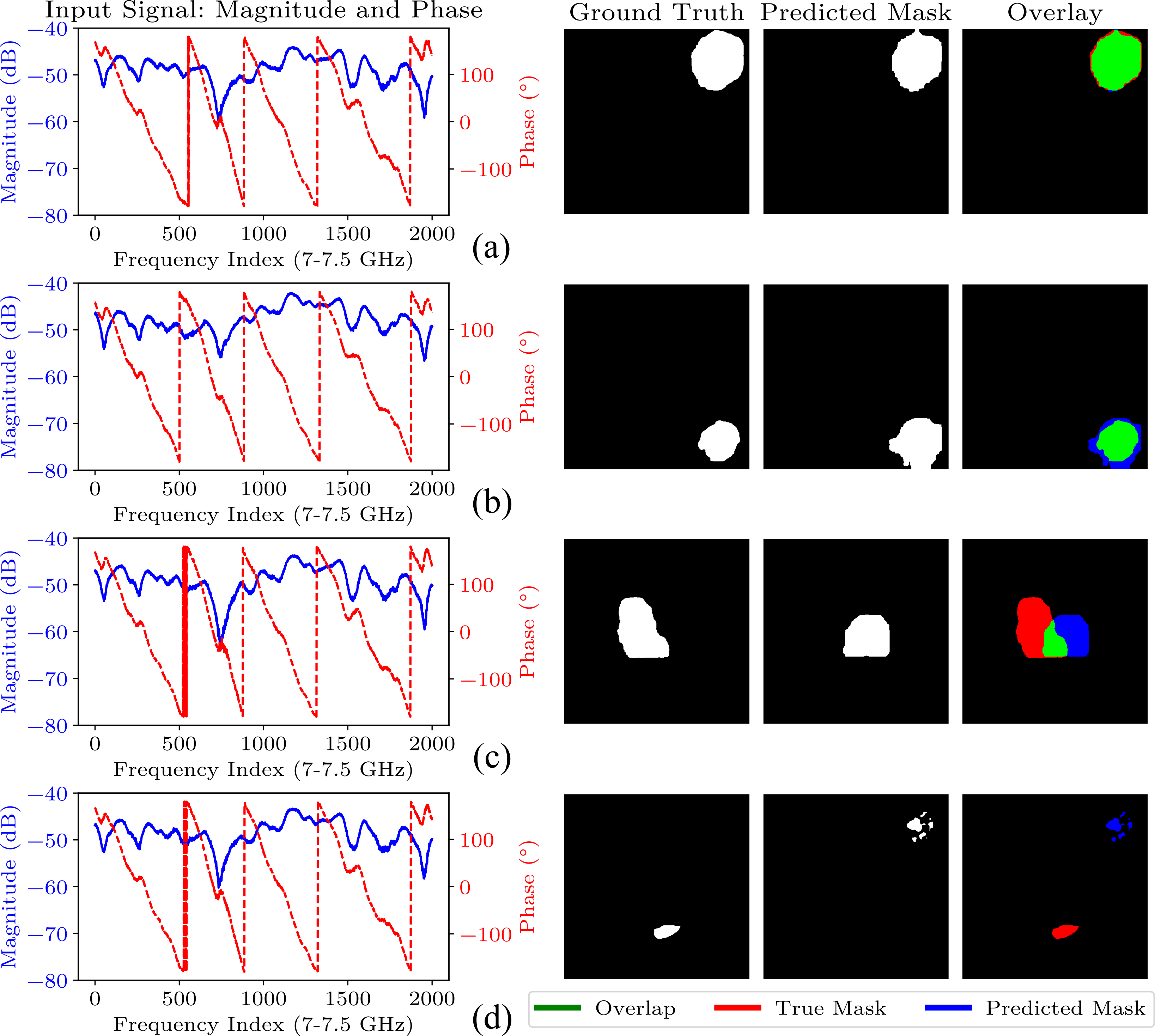
FSS Results

Output: Liquid Type + Spatial Image of the Spill.

We reconstruct an image from a spectral microwave measurement!

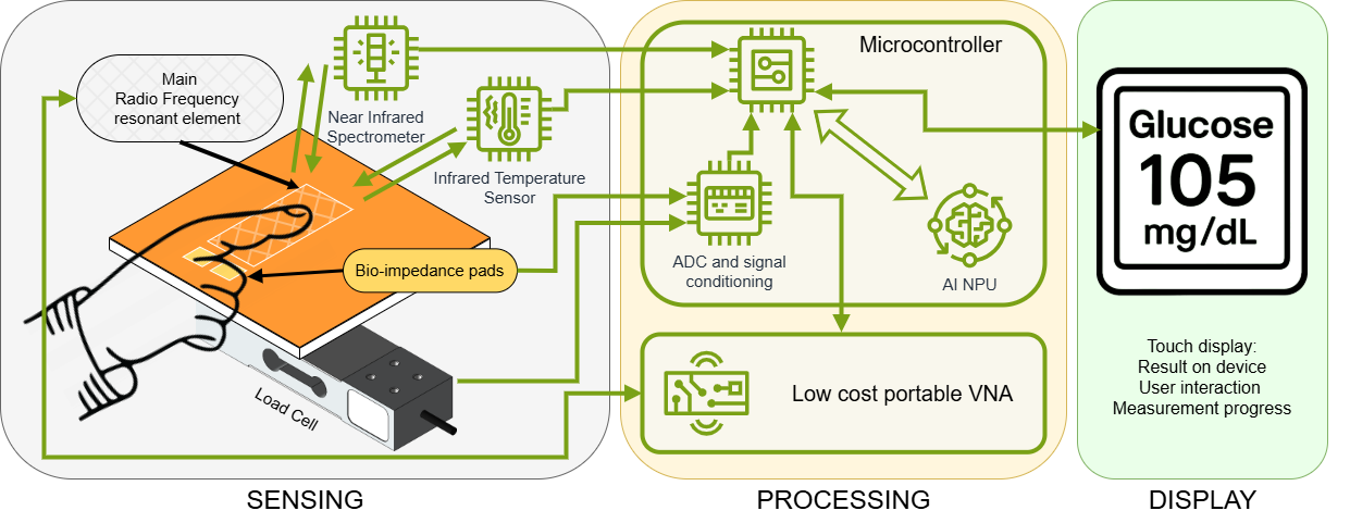
Case 2: Multi-Analyte Sensing

Goal: Measure Glucose, Sodium, and Potassium simultaneously.

Context: Blood analysis.

Challenge: Selectivity. Distinguishing ions from glucose.

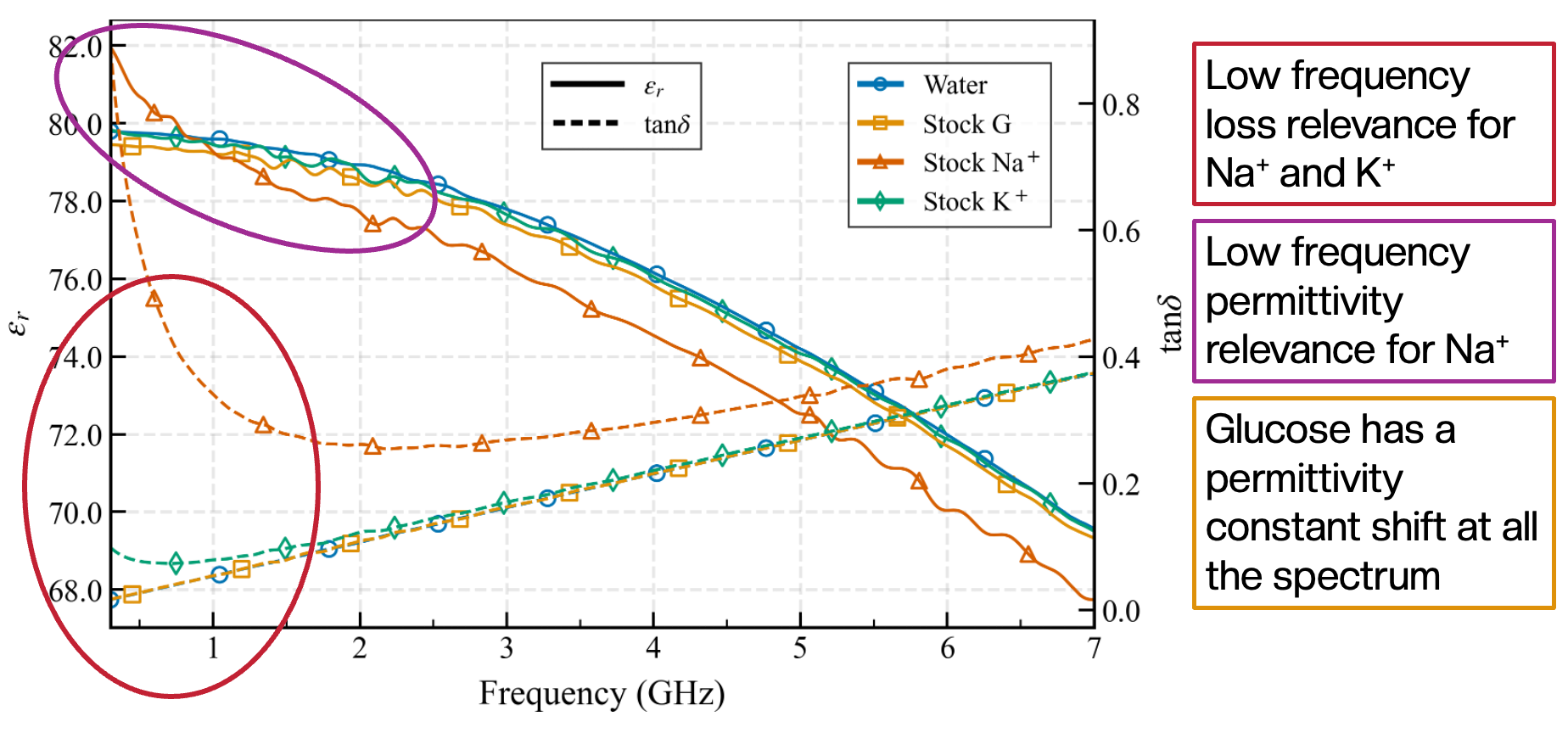
Multi-Analyte Sensor Design

• Sensor: Multi-resonant spiral sensor.
• Feature: Broadband response (100 MHz - 6 GHz).
• Design: Optimized to have features sensitive to different components.

Data Generation

• Automated System: Used the microfluidics system from Objective 2.
• Dataset: Hundreds of mixtures with a set of concentrations.
• Model: CNN + Regression Neural Network.

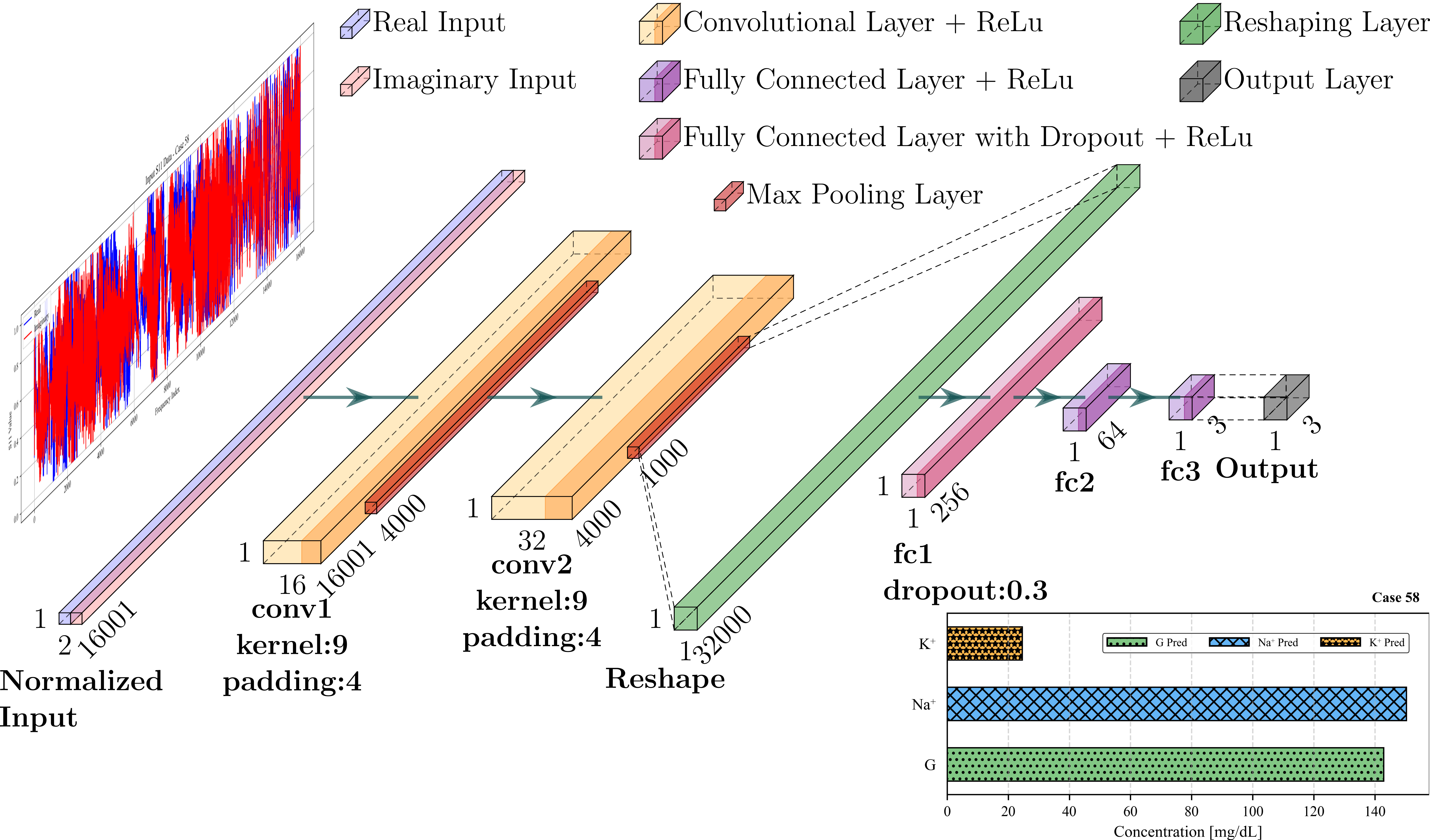
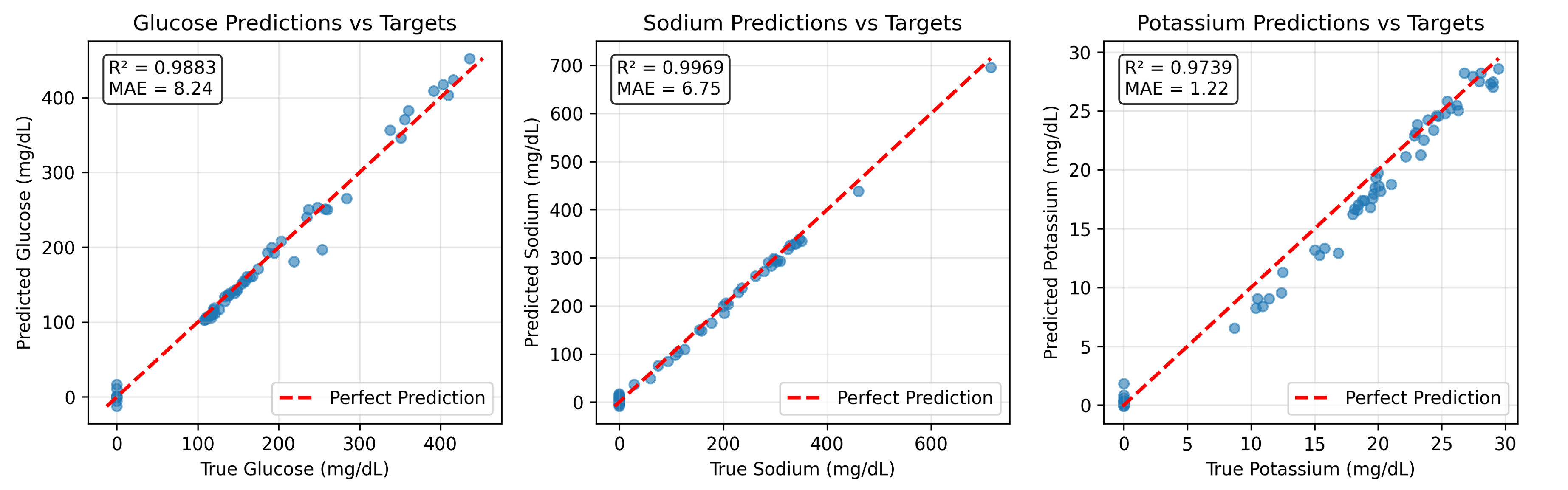
Multi-Analyte Sensor Results

• Model: Regression Neural Network.
• Outcome: Accurate concentrations for all 3 solutes.
• Error: Low enough for clinical screening potential.

Evolution of Performance

Figure of Merit (FoM): Sensitivity / Size.

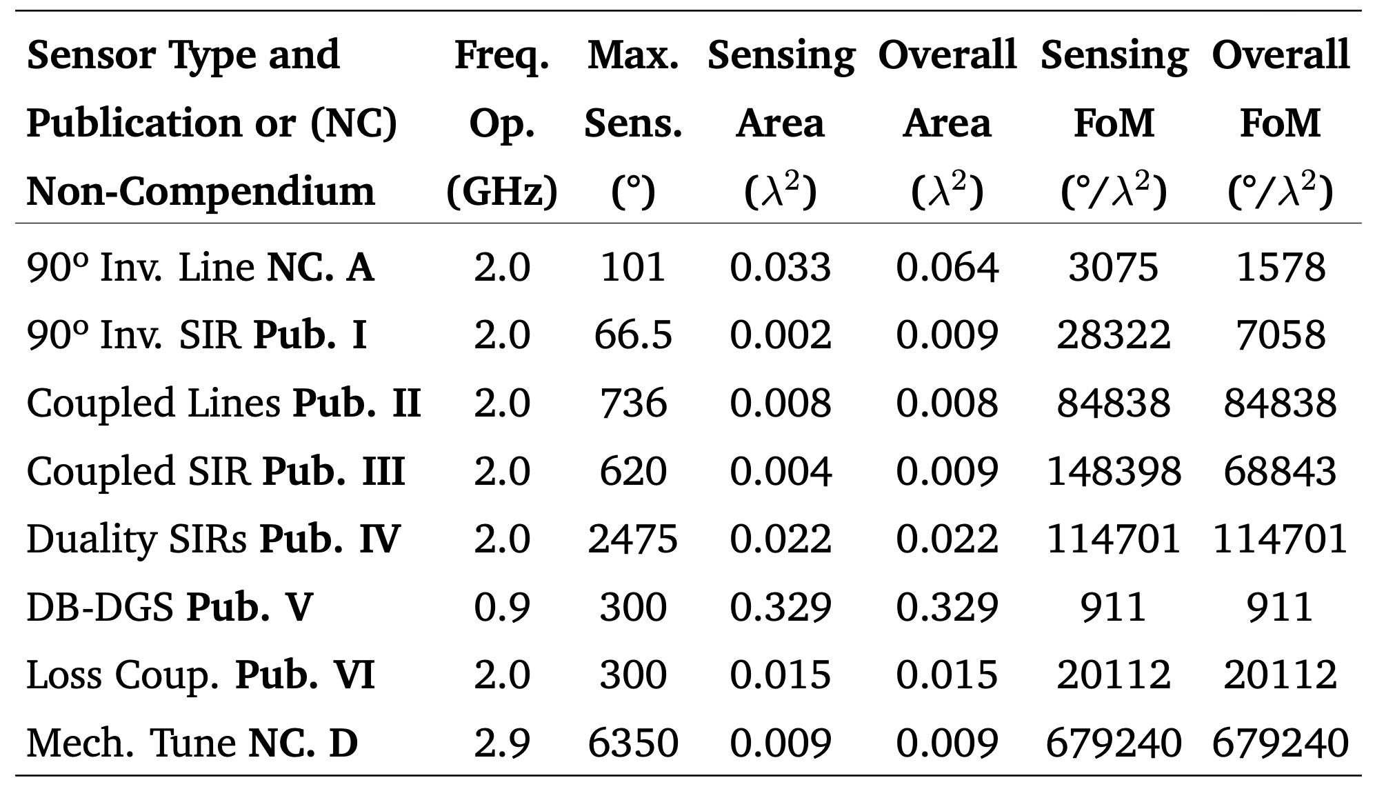
Consistent trend: Higher sensitivity in smaller footprints.

Loss Engineering and Tunability

Paradigm Shift: Loss is usually bad.

Our Finding: Controlled loss can sharpen the phase response.

• Used resistors/JFETs to tune sensitivity.
• Loss as a Design Parameter.
• Enables dynamic adjustment of sensitivity for specific application requirements.

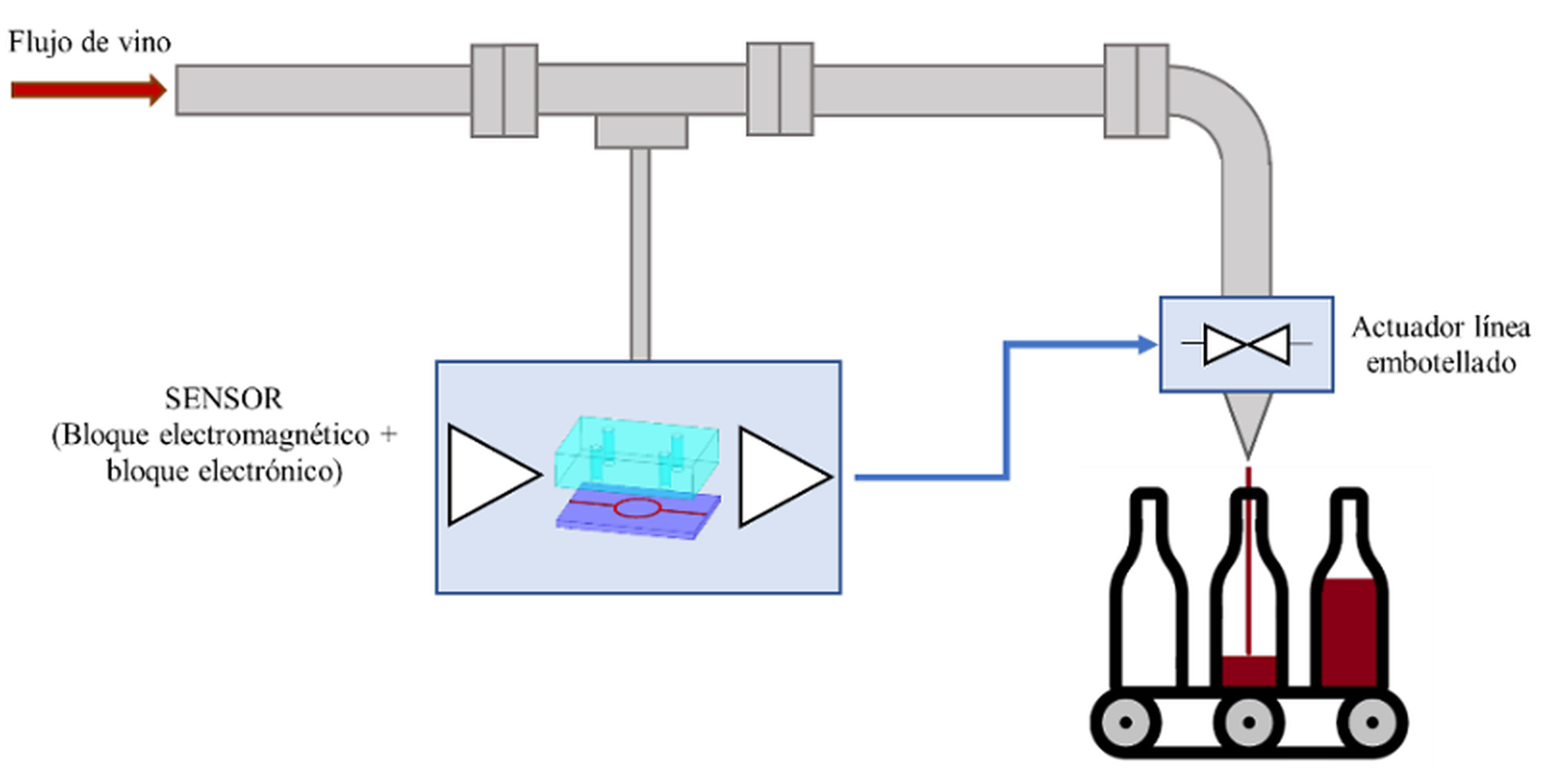
Application: Agrifood

Smart Cellar Project

• Goal: Monitor Clean in Place process to reduce waste.
• Tech: Planar sensors integrated in pipes.
• Partner: Garcia Carrion - CPP Project.

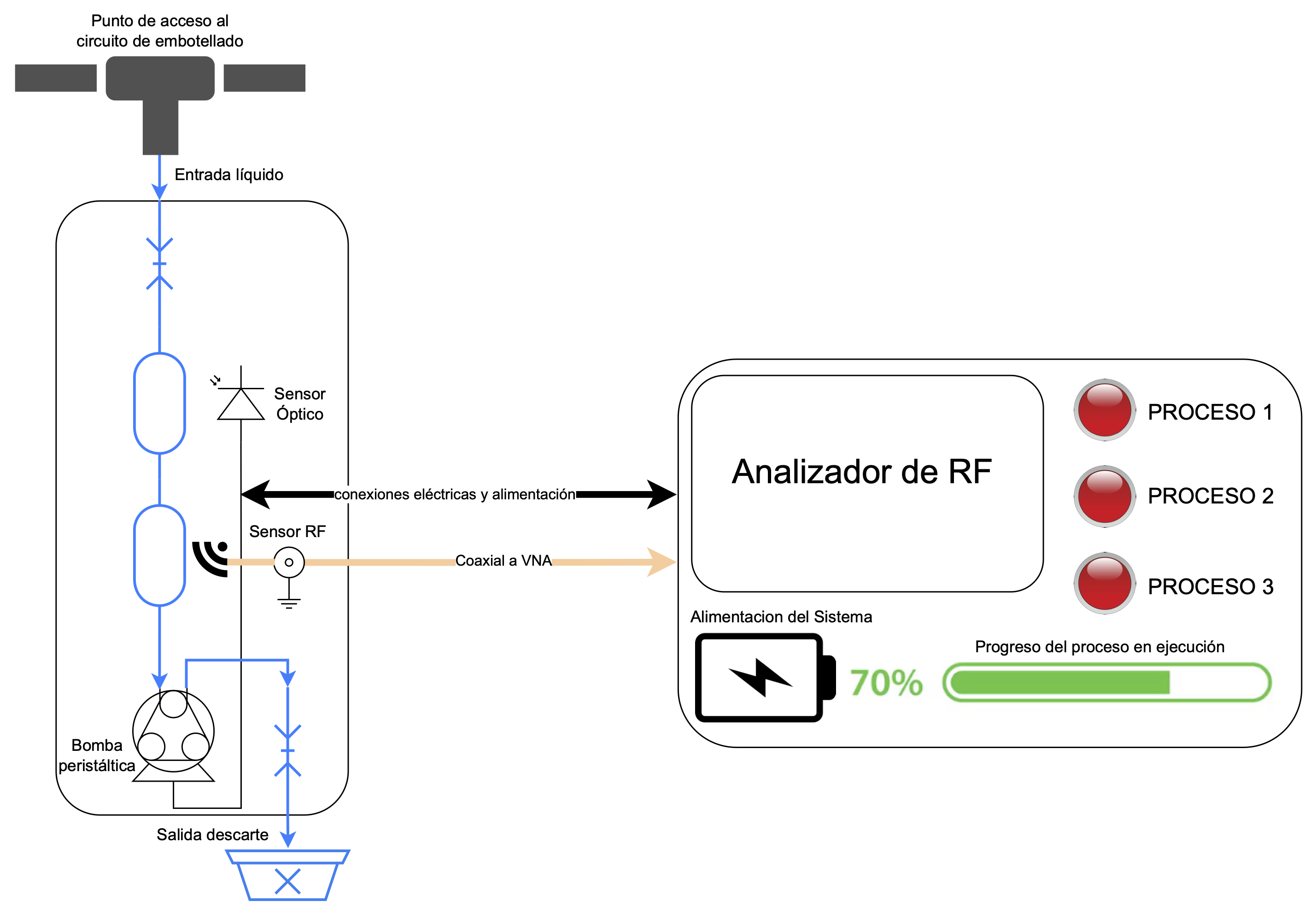
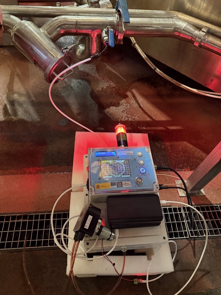
Application: Agrifood

Smart Cellar Project

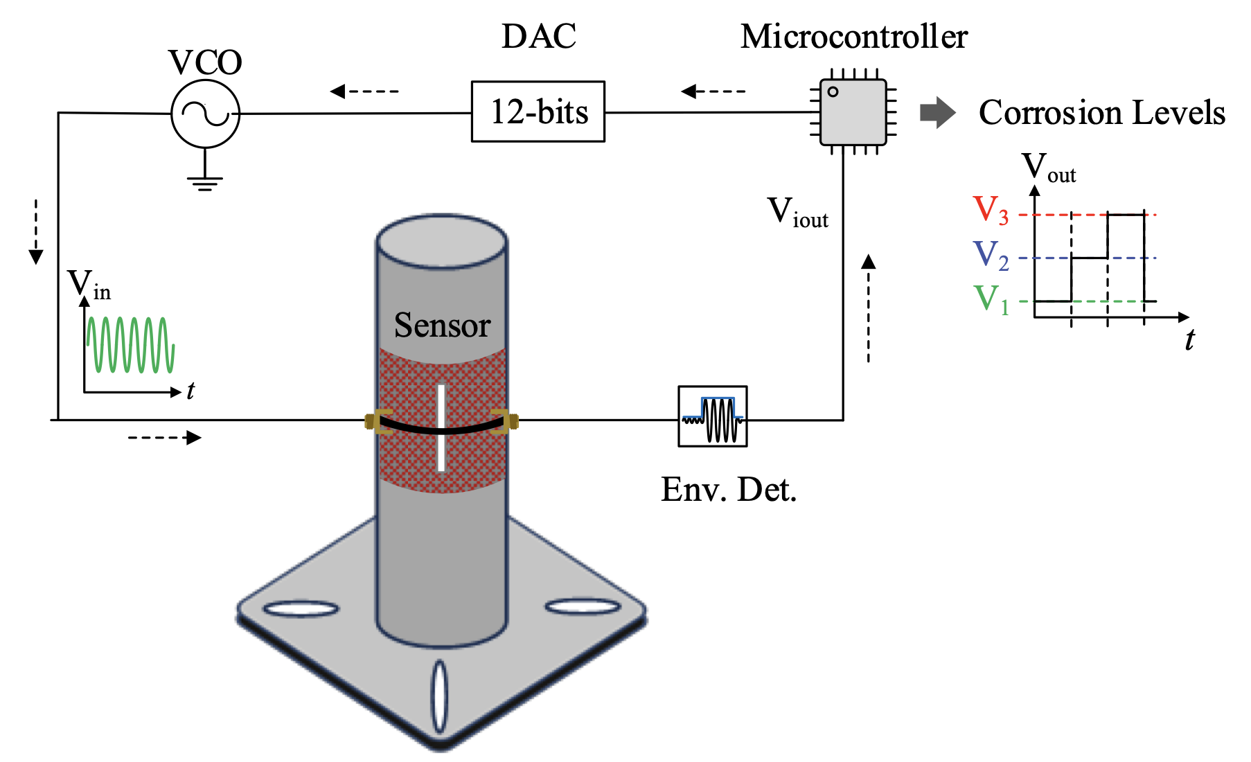
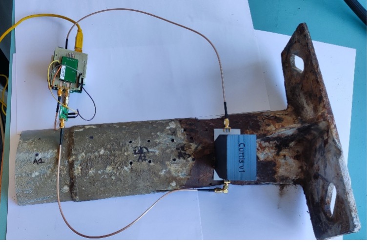
Application: Structural Health

Corrosion Detection

• Goal: Detect rust on street light poles.
• Tech: Resonance-Antiresonance sensors.
• Partner: RUBATEC.

Application: Remote Sensing

WiFi CSI Monitoring

• Goal: Use existing WiFi signals for sensing.
• Tech: AI analysis of Channel State Information.
• Outcome: Passive environmental monitoring.

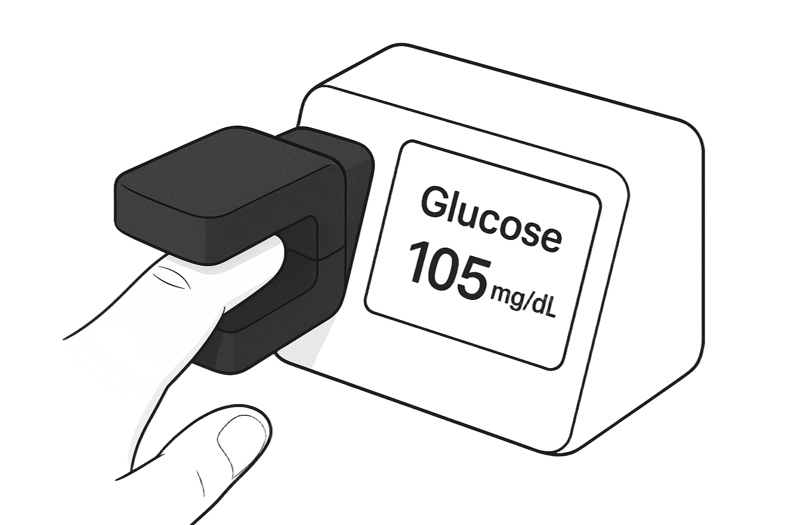
Application: Biomedical

Non-Invasive Glucose

• Goal: Non-invasive measurement of glucose in blood.
• Tech: Multi-Analyte sensor + Sensor Fusion + AI.
• Status: Proof of concept successful.

Future Work: Immediate

Post-Doc Project

• Focus: Non-invasive Glucose Monitoring.
• Plan:
  • In-vivo measurements.
  • Clinical validation.
  • Miniaturization.

Future Work: Long Term

• Generative AI Design: AI designing the sensor.
• Commodity Hardware: Sensing with smartphones/WiFi chips.
• Multi-modal Fusion: Combining microwave with optical/acoustic.

Conclusions

1. Sensitivity: Maximized via phase-slope techniques (Inverters, Coupling, Loss).
2. Methodology: From analytical design to AI-driven paradigm.
3. Impact: Validated in real applications (Liquids, Remote, Bio).

A complete journey from fundamental physics to intelligent systems.

Acknowledgements

Thank you to:

• Prof. Ferran Martín
• GEMMA-CIMITEC Group
• Funding Agencies (FPU, CPP)
• Collaborators (UBC, RUBATEC, Garcia Carrion)
• Family & Friends

Thank You!